GGPlot Installation and Setup
Plot Styles
We are going to open the RStudio Project we created in the last lesson. You can open your project by any of the following three methods:
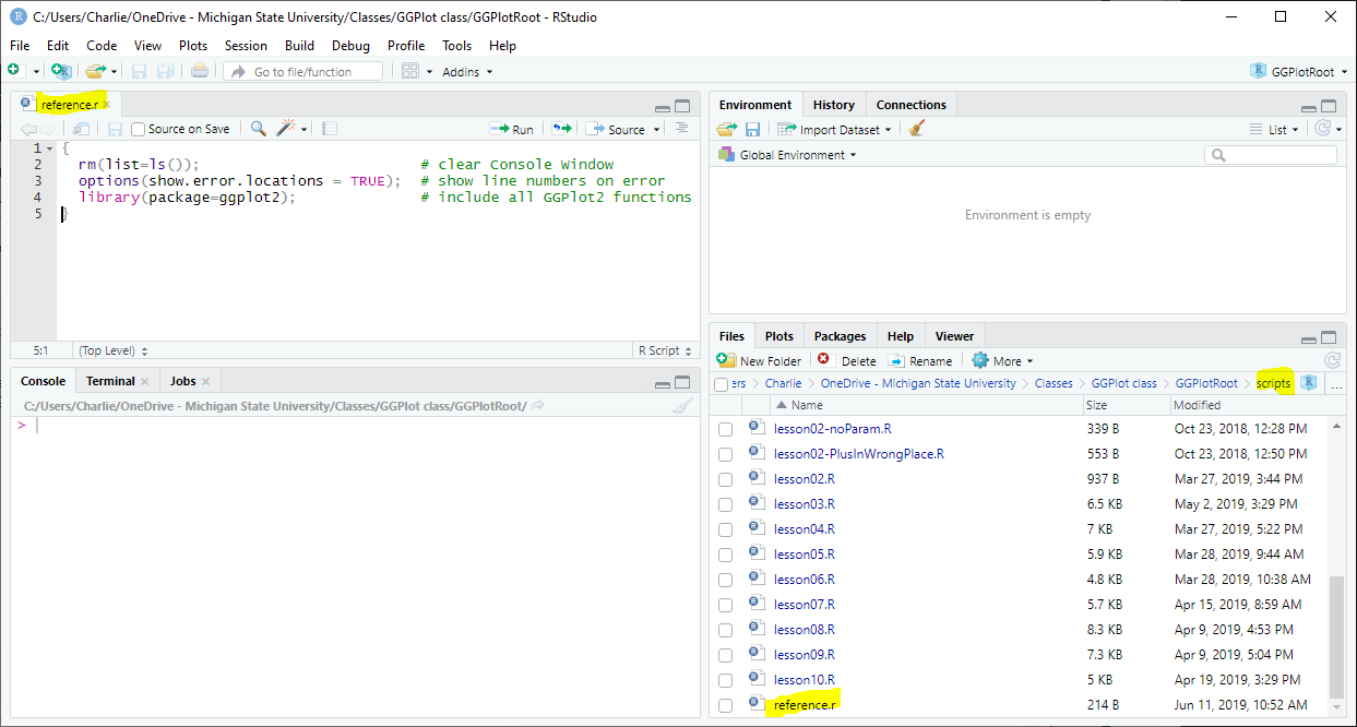
The first script we will create is a reference script, which is a script that is called by other scripts but is not executed on its own. The purpose of a reference script is to contain code used by multiple script files so that the code does not have to be repeated in each of those individual script file. Note: packages from libraries are also examples of reference scripts.
To create a new script in RStudio, click File -> New File -> R Script.
For now the reference script will contain three lines:
Copy the three lines to your new script file and save this script as reference.R inside the scripts folder in your Project (File -> Save as... -> open scripts folder -> click Save) .
The second line of reference.r:
is a good line to always include in your R code because it helps you debug by giving you the line number that the compiler thinks an error is on. However, this error detection does not work within GGPlot code. So, it is of limited use in this class.
A plotting program is not very useful unless it has data. So, we first need to get some data and then set up a script to read in the data.
This website has hundreds of data set that are freely available. We are going to use the data set called Growth of CRAN. The data set gives the number of R Packages that were available each year from 2000 through 2014.
Save the CSV file, called CRANPackages.csv to the data folder inside your Project. It is best to use the operating system's File Explorer/Finder to move the CSV file to the proper folder. Trap: Using Excel to move a CSV file
We are going to start a new script called lesson02.R and use it to read in and plot the data from CRANPackage.csv.
To read in the data from CRANPackages.csv:
Save the script file as lesson02.r inside the scripts folder in your RStudio Project.
We execute lesson02.r by clicking Source (fig ##). Extension: Run vs. Source
The script created the variable packageData, which you can see in the Environment Window (fig ##). packageData is a data frame with 5 columns and 29 rows populated from CRANPackages.csv.
A quick look at the five columns in packageData (fig ##) shows that column 4 contains the number of Packages in CRAN and column 3 contains the corresponding Date.
Next, we will create a scatterplot of Packages (column 4) vs Date (column 3) from packageData.
The code to create a scatterplot using GGPlot is:
Let's Source the script -- the code will be explained in a bit and the overlapping x-axis date labels will be fixed.
Extension: The yellow warning sign
In fig ## I highlighted the parameter names in the code (which, in GGPlot, are also the subcomponents). In this case, the script will still work even if we take out all the parameter names:
This script works because we only used the default parameters for each function and we used the parameters in the same order as they appear in the function.
In this class, we will (almost always) use parameter names because using parameter names:
The one exception where we will not use parameter names is:
instead of
There are multiple functions in R and GGPlot where the parameter name x is used generically as the name for the first parameter in a function. This is not intuitive because x is also used to refer to data that goes on the x-axis.
We will use the parameter name x only when x refers to an axis (line 10 in fig ##: x=Date) but not when x is a generic first-parameter name (line 11 in fig ##: x=plotData).
Let's take a more detailed look at the three lines of code that created the scatterplot in figure ##...
First we initialize the canvas for the plotting area using ggplot() and the data frame we are going to use, packageData:
Next, we add the component, geom_point(), which creates a scatterplot using the Date and Packages columns from packageData:
The ggplot information is saved to a List variable named plotData:
And then plot() is used to display the canvas saved in plotData:
In GGPlot, you initialize a canvas and then add components (often called layers) to the canvas. The + symbol is used to add components. In the above example (fig ##), there is the initializing canvas function and one component:
1) ggplot() is used to initialize a GGPlot canvas with the data from the data frame:
2) geom_point() is a plotting component that creates a scatterplot
All plotting components in GGPlot contain a subcomponent called mapping. mapping is used to describe the relationship between the data and the plot. Or, another way to put it, mapping describes what data gets represented on the plot (e.g., Date and Packages) and how the data gets represented (e.g., Date on x-axis, Packages on y-axis):
The mapping is set to a mapping element called an aesthetic (aes). The concept of an aesthetic comes into play when we are generating legends and creating data categories, which we will talk about in future lessons. In the meantime, it is probably easier to just think of aes as a mapping element.
Let's say we want to make the three following modifications to the plot:
To do this we will add three new components to the canvas:
We add components using ( + ).
Trap: putting the ( + ) on the next line
When we search in the Help tab for ggtitle() (fig ##) we see that it has two subcomponents (or parameters) to change:
scale_y_continuous() is the component used when you want to modify a y-axis that has continuous values. There are many subcomponents (fig ##) that can be changed in scale_y_continuous(). We modified one subcomponent, breaks, by setting it to a sequence from 0 to 6000 and the tick marks were placed at intervals of 500. Note: waiver(), which is used as a default value for many of the subcomponents, is a somewhat unintuituve way of saying to use the values calculated by the plotting function (i.e. default values).
In this example we changed one subcomponent in theme() called axis.text.x and set it to a element_text() that modifies the text by rotating it to an angle of 90 degrees and right-justifying the text (hjust=1). Note: hjust=0 left-justifies the text, hjust=0.5 centers the text.
theme() is probably the most used component in GGPlot and we could spend a whole class going through all the subcomponents of theme(). Broadly speaking, theme() is used to make modifications to the canvas (the plots and the background) that are not data related. We will be using theme() a lot more in future lessons and talking more about elements (e.g., element_text()).
A good place to find more information about components in GGPlot is the Help tab in the lower-right corner of RStudio. The Help tab provides information directly from https://ggplot2.tidyverse.org/reference/, which is the official webpage for GGPlot.
Create a scatterplot:
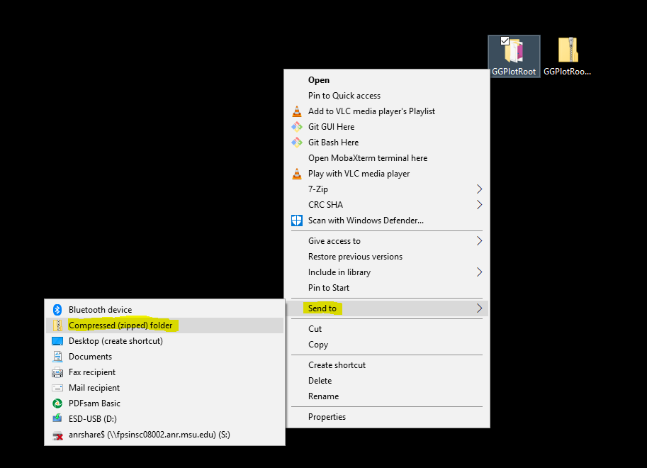
Windows: Zip your Root Folder (fig ##):

Mac: Zip your Root Folder:
An RStudio Project takes the whole RStudio window -- also called an RStudio Session. If you want to open up a second RStudio Project, you need to start a new RStudio Session (i.e., a new window). This can be dome by clicking File -> Open Project in New Session.
RStudio considers only files saved within the Root Folder (and subfolders) of the Project to be a part of the Project. You can create a script file that is independent of the RStudio Project you are working on, you just need to save the script file outside of the Project's Root Folder.
On many computers, Microsoft Excel is the default application for opening CSV files -- so double-clicking on a CSV file opens it in Excel. So, it is common for people to open a CSV file in Excel and then save it to a different folder. There are a couple of issues with using Excel to move CSV files:
You should not use Excel to move a CSV. Instead, use the system's File Explorer (Windows) / Finder (Mac) to move the file. You can also safely open the CSV file in RStudio and save it to another location.
Technically speaking, the difference between Run and Source is:
The real difference lies in a historical discussion of scripting vs. programming, which is a discussion beyond this class. Suffice to say, R was originally intended to be a quick-and-dirty scripting language where users could immediately pull in data and produce a plot or perform statistical analysis. Using this method, an R-user would produce and execute one line of code at a time using the equivalent of the Run button.
As R has grown, the focus has shifted into developing well-structured code that can be easily shared, tweaked, and reused -- similar to a modern programming language like C. Using this method, an R-user would produce a full script and execute it all using the equivalent of the Source button. This is the method we will be using in this class.
The ( + ) commands strings together the components of a GGPlot. A common mistake is to put the ( + ) at the beginning of the following line:
This will result in an error and a surprisingly wise assessment of the problem fro the R debugger.
The reason for this error is that R thinks that line 5:
is a fully-formed and completed command
And R does not understand why line 6 starts a new command with a ( + )
A ( + ) at the end of a line tells R to append the next line to the current line. A ( + ) at the beginning of a line tells R to perform the mathematical operation addition.
When you are working in GGPlot and have debugging features turned on in RStudio, you will almost always see multiple yellow warning signs on the side of your code (fig ##). The warning no symbol named 'Date' in scope means that RStudio does not recognize Date as a variable or a function. This is because Date is a variable within the GGPlot function geom_point(), and the debugger is not sophisticated enough to always search through the GGPlot functions.
Unfortunately, this is just a limitation of the RStudio debugger.