Software tools for Maximum Likelihood Estimation:MB

Lesson 2 - first RTMB & Derivatives
Click here to view presentation online

Jim Bence

1 December 2023

Outline:

• Demos of using nlminb and RTMB to estimate parameters
• Explanation of what happened in RTMB
• Simple exercise adapting RTMB example
• All that derivative stuff
  • derivatives, partial derivatives, second derivatives, cross derivatives (aka mixed second derivatives), gradient vector and Hessian
• Methods to calculate/appoximate derivatives
• Exercise: finite difference derivatives
• How the Hessian and gradient vector are used
• RTMB Nonlinear regression vonb example

Demos of estimating the mean the hard way

• Just using nlminb

• Using RTMB

“Magic” when we used MakeADFun in RTMB

• Converts your parameter list and NLL function into new inputs for nlminb (and lots of hidden stuff)

  • obj$par: your list of starting values as vector

  • obj$fn: function pointing to memory location where NLL function result is stored

  • obj$gr: function pointing to memory location where gradient stored

• IMPORTANT! obj$fn and obj$gr use hidden copy (created by MakeADFun) of any variables used in your NLL function

Exercise - change model to assume gamma rather than normal (in breakout groups)

What is a derivative

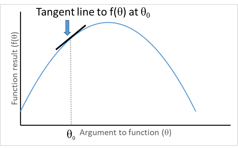
\[ \frac{d f(\theta)}{d \theta}=\lim h \rightarrow 0 \frac{f(\theta+h)-f(\theta)}{h} \]

Partial derivative

Function with multiple arguments but we treat all but one of them as constants, and calculate derivative with respect to just one! E.g.,

\[ \frac{\partial f}{\partial \theta_{2}}=\lim h \rightarrow 0 \frac{f\left(\theta_{1}, \theta_{2}+h, \theta_{3}\right)-f\left(\theta_{1}, \theta_{2}, \theta_{3}\right)}{h} \]

Second derivative

Just a derivative of a derivative

\[ \frac{\partial^{2} f}{\partial \theta^{2}}=\frac{\partial \frac{\partial f}{\theta}}{\partial \theta} \]

Visualizing second derivatives

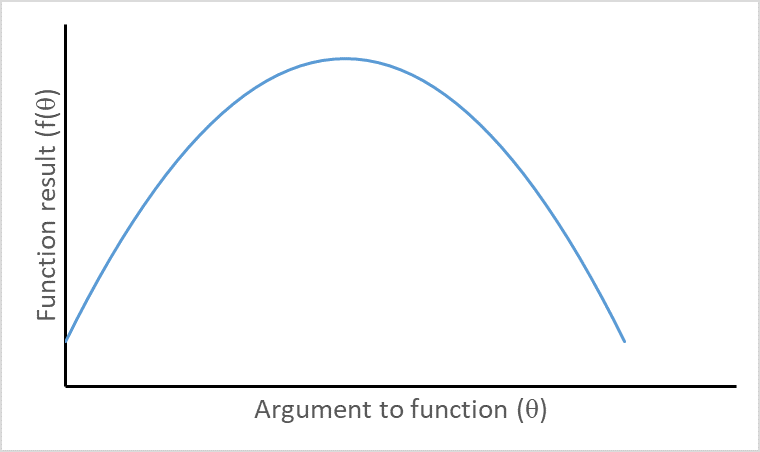
Concave function with negative second derivative

Visualizing second derivatives

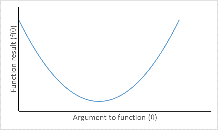
Convex function with positive second derivative

Cross derivative (mixed second derivs)

\[ \frac{\partial^{2} f}{\partial \theta_{1} \partial \theta_{2}}=\frac{\partial \frac{\partial f}{\partial \theta_{1}}}{\partial \theta_{2}} \]

An important and convenient fact:

\[ \frac{\partial^{2} f}{\partial \theta_{1} \partial \theta_{2}}=\frac{\partial^{2} f}{\partial \theta_{2} \partial \theta_{1}} \]

Methods for calculating derivatives

• Analytical derivatives. Gold standard but not available for many complex models.

• Finite difference methods. Intuitive but slow and propogate errors.

• Automatic differentiation. Fast and accurate but requires specialized software.

Finite difference derivatives

Widely used, e.g., default of nlminb and Excel solver

Forward difference

\[ \partial f / \partial \theta_{i}=\frac{f\left(\theta_{i}+h\right)-f\left(\theta_{i}\right)}{h} \]

h is semi-arbitrary but small relative to \(\theta_i\).

Central differences

\[ \partial f / \partial \theta_{i}=\frac{f\left(\theta_{i}+h/2\right)-f\left(\theta_{i}-h/2\right)}{h} \]

Exercise - finite difference derivatives

• For g(x) = a + b X + sin X, use finite difference methods to calculate the derivative of g(X) with respect to (wrt) X
  • for x=1, with a=2 and b=0.5. (answer approximately 1.040)
  • Repeat for x=2, a=1, and b=1. Answer approximately 0.5839.
• For a=2, b=0.5, x=1, and same function, use finite differences to find the second derivative wrt x (answer approximately -0.8415)

Automatic differentiation

• Uses repeated applications of chain rule: \(\partial z / \partial \theta=[\partial z / \partial y][\partial y / \partial \theta]\)

• Simplest case. \(y=f(\theta)\), \(z=g(y)\), i.e., \(z=g(f(\theta))\)

• General case we care about:

  \[ NLL=f_1(f_2(f_3(...f_k(\theta)...))) \]

Gradient

Just a fancy term to mean the vector of derivatives of the NLL function with respect to each parameters (so if k parameters, then k elements)

\[ g=\left\{\partial f / \partial \theta_{1}, \partial f / \partial \theta_{2}, \ldots \partial f / \partial \theta_{k}\right\}^{T} \]

Hessian - a square symmetric marix

\[ H=\left[\begin{array}{cccc}\partial^{2} f / \partial \theta_{1}^{2} & \partial^{2} f / \partial \theta_{1} \partial \theta_{2} & \ldots & \partial^{2} f / \partial \theta_{1} \partial \theta_{k} \\\partial^{2} f / \partial \theta_{2} \partial \theta_{1} & \partial^{2} f / \partial \theta_{2}^{2} & \ldots & \partial^{2} f / \partial \theta_{2} \partial \theta_{k} \\\ldots & \ldots & \ldots & \ldots \\\partial^{2} f / \partial \theta_{k} \partial \theta_{1} & \partial^{2} f / \partial \theta_{k} \partial \theta_{2} & \ldots & \partial^{2} f / \partial \theta_{k}^{2}\end{array}\right] \]

\[ h_{i,j}=h_{j,i}=\frac{\partial^{2} f}{\partial \theta_{i} \partial \theta_{j}}=\frac{\partial^{2} f}{\partial \theta_{j} \partial \theta_{i}} \]

If the NLL were a quadratic function as it would be for linear normal model…

\[ \theta_{\text {min }}=\theta_{\text {start }}+H^{-1} g \]

where \(H^{-1}\) in the matrix inverse of \(H\) and \(H^{-1}g\) is the product of the inverse of the Hessian and the gradient

Because our models generally not normal and linear, iterative searches…

1. specify starting values for parameters, \(\underline{\theta_0}\)

2. Replace \(\underline{\theta_0}\) by \(\underline{\theta_1}=\underline{\theta_0}+\delta_0\)

3. Check gradient and Hessian and if at a minimum stop otherwise…

4. Return to step 2 but each time \(\underline{\theta_{i+1}}=\underline{\theta_i}+\delta_i\)

Newton step: \(\underline{\delta}_{i}=H^{-1} \mathrm{\underline{g}}\) evaluated at current params

Quasi-Newton method uses \(\underline{\delta}_{i}=\lambda H^{-1} \mathrm{\underline{g}}\) with Hessian approximated using search path, and \(\lambda\) a number less than 1

Using the Hessian to calculate asymptotic standard errors

• First some reminders

  • Parameter estimates are random variates that result from estimators (random variables)

  • The variance describes the variability of results from applying the estimation method, namely the expected squared deviation between an estimator and its expected value

  • What we report as a standard error for a parameter is the square-root of this variance.

The variance-covariance matrix

\[ \Sigma=\begin{array}{cccc}\sigma_{1}^{2} & \sigma_{1,2} & \ldots & \sigma_{1, k} \\\sigma_{2, 1} & \sigma_{2}^{2} & \ldots & \sigma_{2, k} \\\ldots & \ldots & \ldots & \ldots \\\sigma_{k, 1} & \sigma_{k, 2} & \ldots & \sigma_{k}^{2}\end{array} \]

The asymptotic variance-covariance matrix

\[ \hat{\Sigma}=H^{-1} \]

• Square-root of diagonal gives standard errors

• Off-diagonals are covariances

• The Hessian needs to be positive definite for the calculation

• If the Hessian is not positive definite its a problem!

• Delta method used to obtain SEs for derived quantities (using \(\hat{\Sigma}\))

Musky vonB example

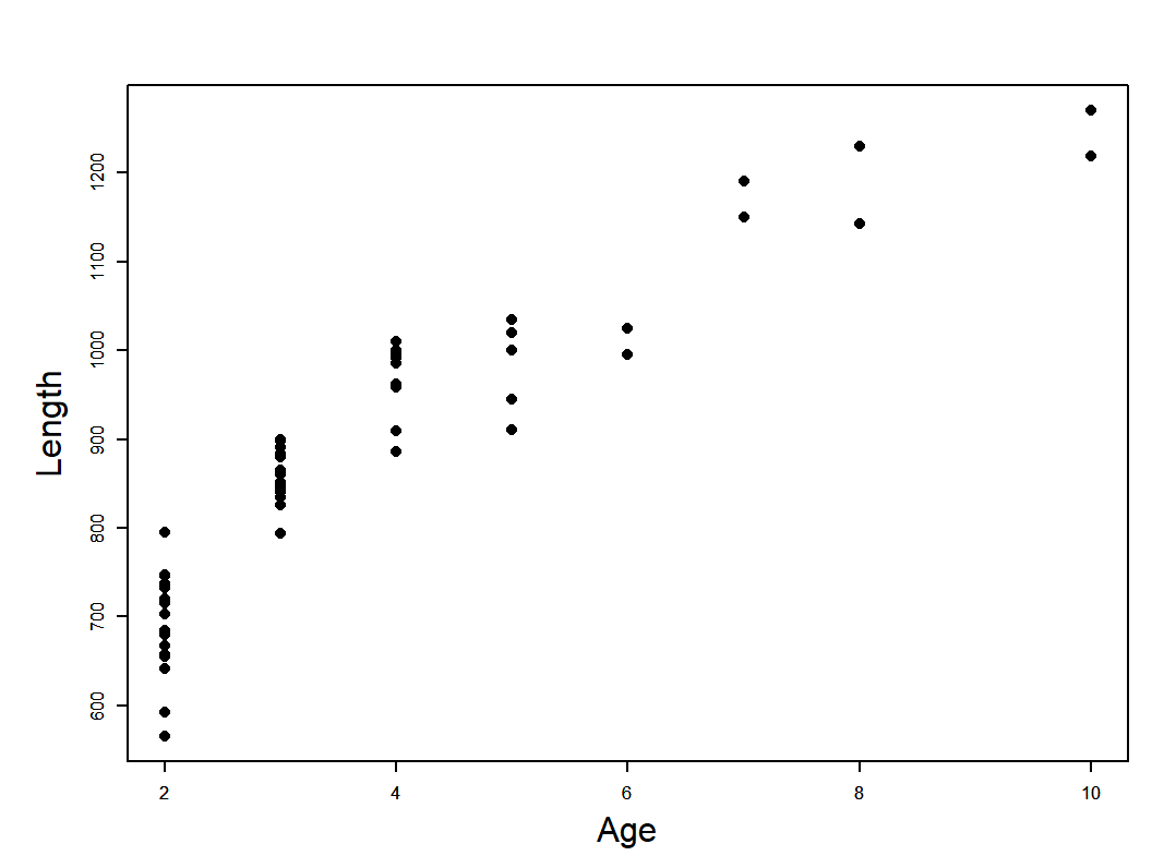
musky_vonb.dat

von Bertalanffy model

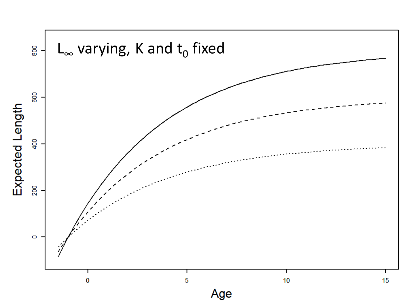
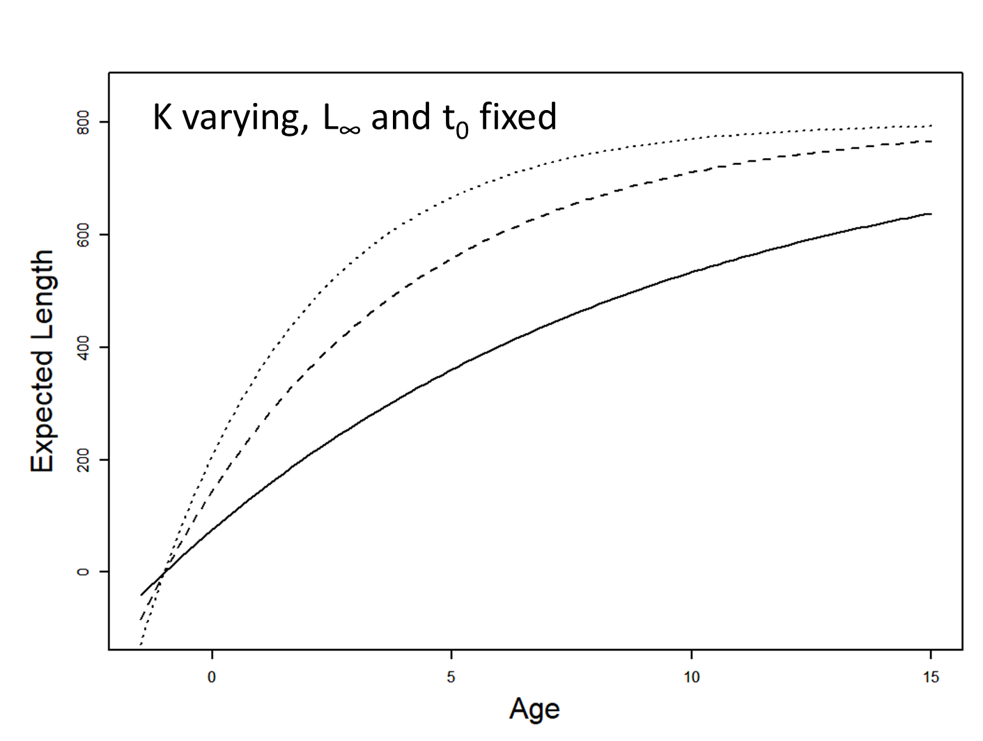
\[ \begin{array}{l}L_{i}=L_{\infty}\left(1-e^{-K\left(a_{i}-t_{0}\right)}\right)+\varepsilon_{i} \\\varepsilon_{i} \stackrel{i i d}{\sim} N\left(0, \sigma^{2}\right)\end{array} \]

\[ L_{i} \sim N\left(L_{a_{i}}, \sigma^{2}\right) \]

Influence of Linf

Influence of K

Musky vonB setup code

library(RTMB);

gmRdat = read.table("lesson2/data/musky_vonb.dat",head=T);

#Set up the data and starting value of parameters for RTMB
gmdat = list(len_obs=gmRdat[,"Length"],age=gmRdat[,"Age"]);
gmpar = list(log_linf=7,log_vbk=-1.6,t0=0,log_sd=4);

code for NLL for Musky vonb example

NLL_fun = function(par_lst){
  getAll(gmdat,par_lst);
  linf = exp(log_linf);
  vbk = exp(log_vbk);
  sd = exp(log_sd);
  len_pred = linf * (1 - exp(-vbk * (age - t0)));
  nll = -sum(dnorm(len_obs, len_pred, sd, TRUE));
  atage_pred = linf * (1 - exp(-vbk * ((1:11) - t0)))
  REPORT(atage_pred);
  nll
}

Create model object and print predicted lengths before fitting model

obj <- MakeADFun(NLL_fun,gmpar);

GMreport=obj$report();
GMreport

$atage_pred
 [1] 200.4870 364.3209 498.2026 607.6080 697.0118 770.0708 829.7731 878.5606
 [9] 918.4287 951.0082 977.6314

fit the model

fit = nlminb(obj$par, obj$fn, obj$gr);

outer mgc:  3572.344 
outer mgc:  115.0372 
outer mgc:  306.8376 
outer mgc:  101.0471 
outer mgc:  30.69436 
outer mgc:  135.1418 
outer mgc:  120.5931 
outer mgc:  25.99566 
outer mgc:  197.1401 
outer mgc:  122.5854 
outer mgc:  66.52428 
outer mgc:  36.54847 
outer mgc:  3.778352 
outer mgc:  19.59957 
outer mgc:  1.539833 
outer mgc:  0.6958294 
outer mgc:  0.239123 
outer mgc:  0.1362159 
outer mgc:  0.02895874 
outer mgc:  0.001790128 
outer mgc:  0.0001970265 

Get parameter uncertainties and convergence diagnostics

sdr = sdreport(obj);

outer mgc:  0.0001970265 
outer mgc:  19.77567 
outer mgc:  19.71682 
outer mgc:  9.178336 
outer mgc:  9.171702 
outer mgc:  2.35869 
outer mgc:  2.358392 
outer mgc:  0.1198859 
outer mgc:  0.1201142 

sdr #summary(sdr)

sdreport(.) result
           Estimate Std. Error
log_linf  7.1488714 0.04083255
log_vbk  -1.2456407 0.16950408
t0       -0.7710237 0.35092437
log_sd    3.8876390 0.09128707
Maximum gradient component: 0.0001970265 

Predicted lengths at age after model fitting

GMreport = obj$report();
GMreport;

$atage_pred
 [1]  508.1491  699.3217  842.6904  950.2090 1030.8420 1091.3122 1136.6614
 [8] 1170.6709 1196.1760 1215.3035 1229.6480

vonB Exercises

• Change REPORT(atage_pred) to ADREPORT(atage_pred) and look at sdreport and summary of the sdreport

• Calculate a new variable equal to vbk*linf as ADREPORT

• Change the model so data are assumed gamma distributed (with expected value given by vonB equation and constant variance)