library(tidyverse) # for plotting
# install.packages("devtools")
# devtools::install_github("QFCatMSU/gg-qfc")
library(ggqfc) # formatting, run previous 2 lines for first gg-qfc install

y <- 2 # successes
n <- 30 # trials
eps <- 1e-6 # buffer because theta must lie within [0,1]
theta <- seq(eps, 1 - eps, length.out = 1e4) # sequence to thetas to try
logLike <- y * log(theta) + (n - y) * log(1 - theta) # plug thetas into pmf
MLE <- theta[which.max(logLike)] # maximum likelihood estimate
my_data <- data.frame(logLike, theta) # for plottingApplied Bayesian Modeling for Natural Resource Management
FW 891
Click here to view presentation online
28 August 2023
My background
Bayesian examples from my work
- Decline was not statistically significant (frequentist)
- 88% chance of population decline (Bayesian)
Bayesian examples from my work

Examples from my work cont’d
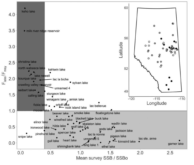
- Reconstructing population dynamics across landscapes
Examples from my work cont’d
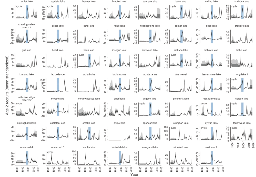
Examples from my work cont’d
Software, implementation, website
- We are primarily going to use R and Stan
- Recommend Rstudio
- Lectures and code will be available through GitHub
- You do not need to know how to use GitHub, but that is where you can find code and presentations

![]()

![]()


Stan is not:


What is Stan, why use it?
Stan is a state-of-the-art platform for statistical modeling and high-performance statistical computation
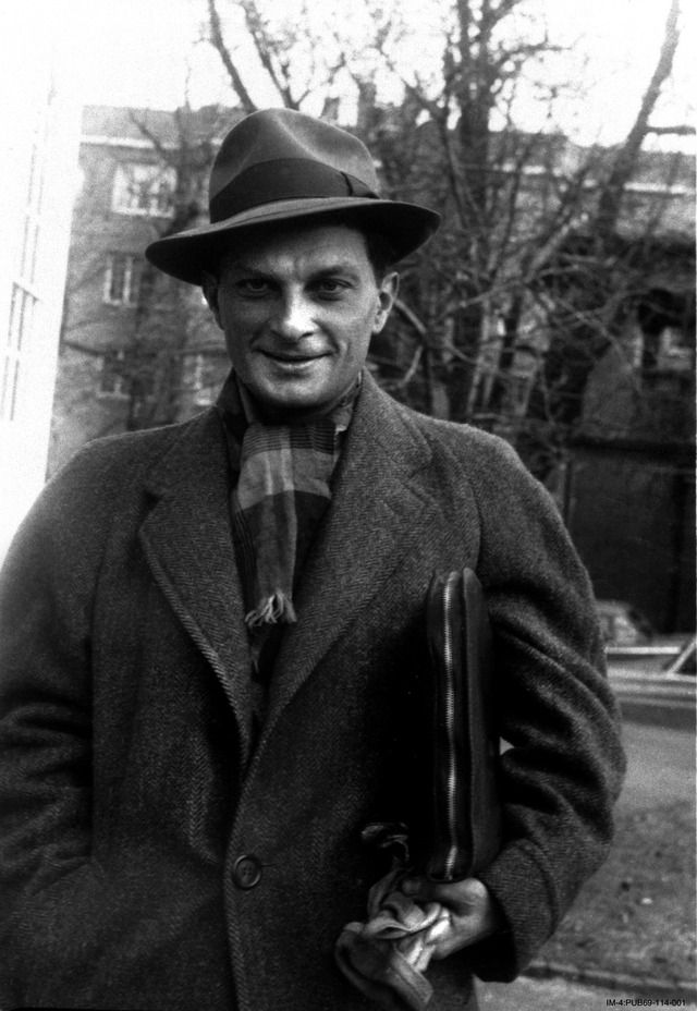
Named after Stanislav Ulam
Unique class of algorithms (HMC, NUTS), scales well
Cannot do everything (discrete unknowns)


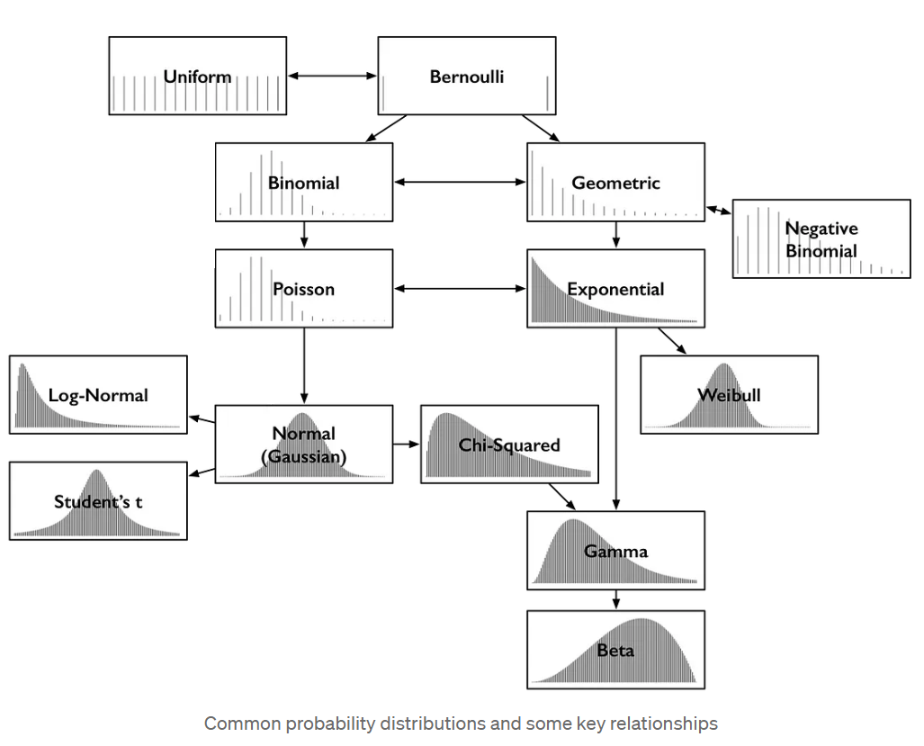
Some common statistical distributions
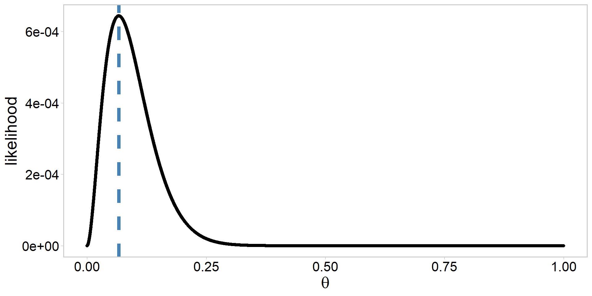
Alabama sneak turtles: log-likelihood

Moving from log-likelihood to likelihood
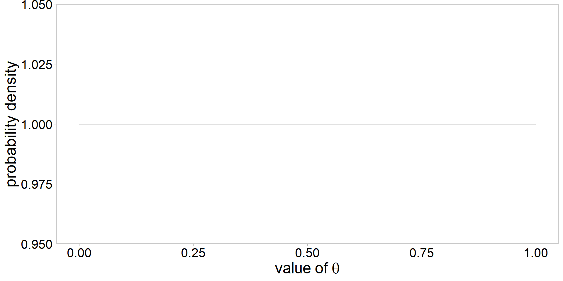
Visualizing a \(\mathrm{beta}(\alpha, \beta)\) prior
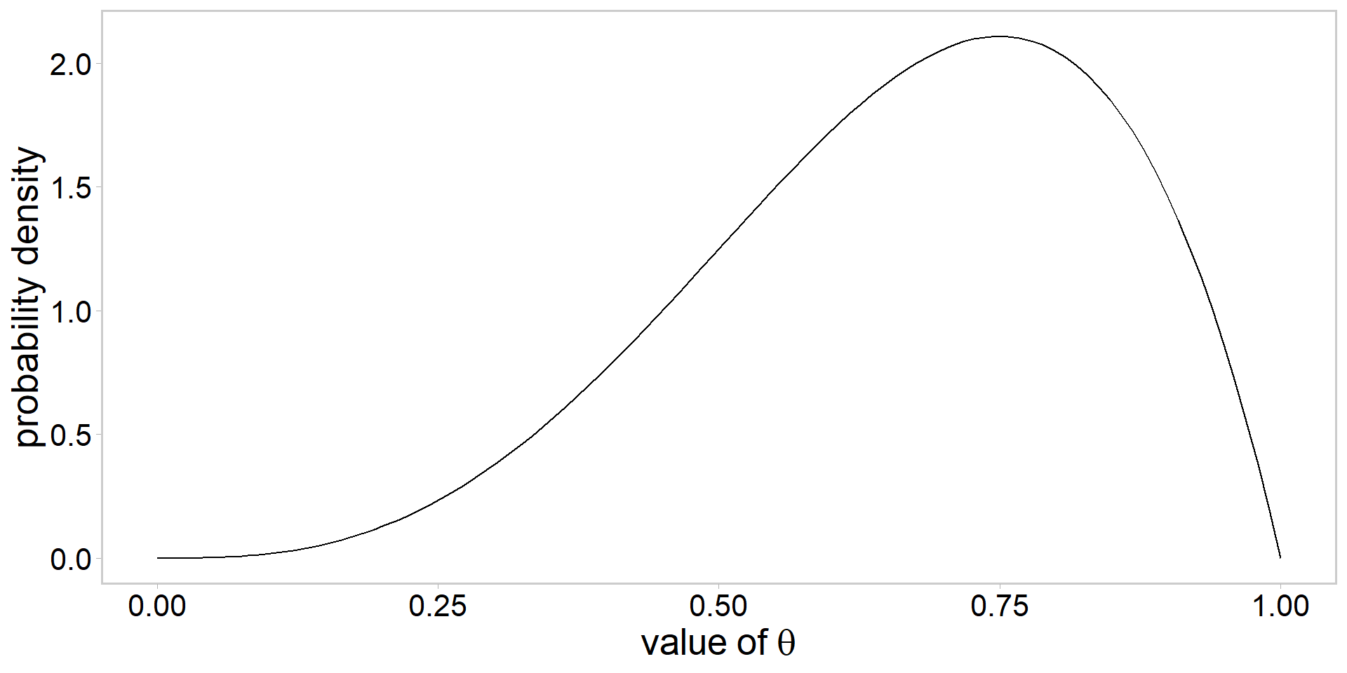
- always a good idea to visualize
Visualizing a \(\mathrm{beta}(\alpha, \beta)\) prior
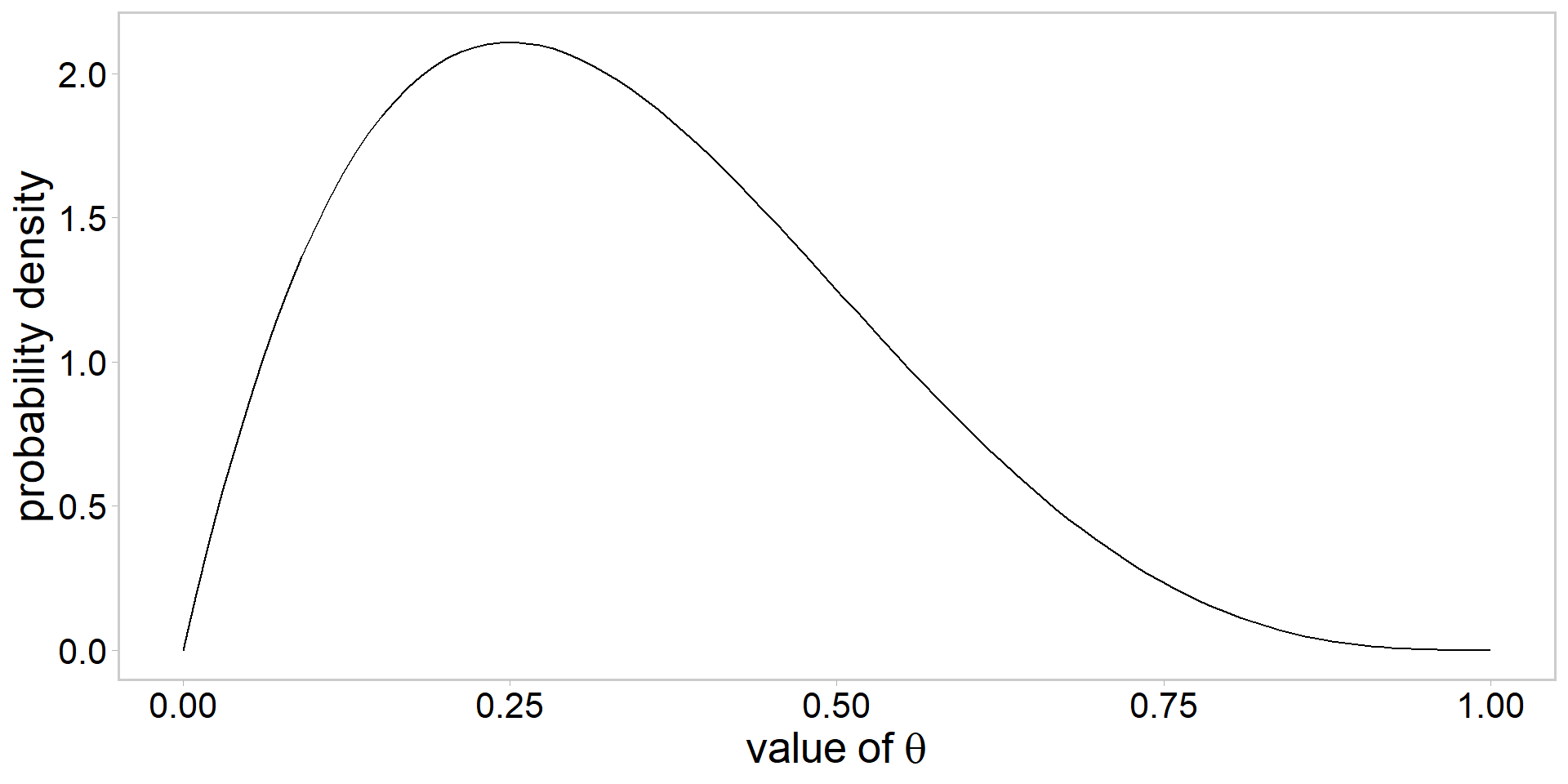
- always a good idea to visualize
Visualizing a \(\mathrm{beta}(\alpha, \beta)\) prior
- always a good idea to visualize
Visualizing a \(\mathrm{beta}(\alpha, \beta)\) prior
- always a good idea to visualize
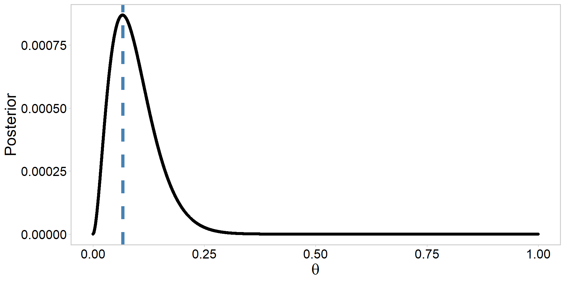
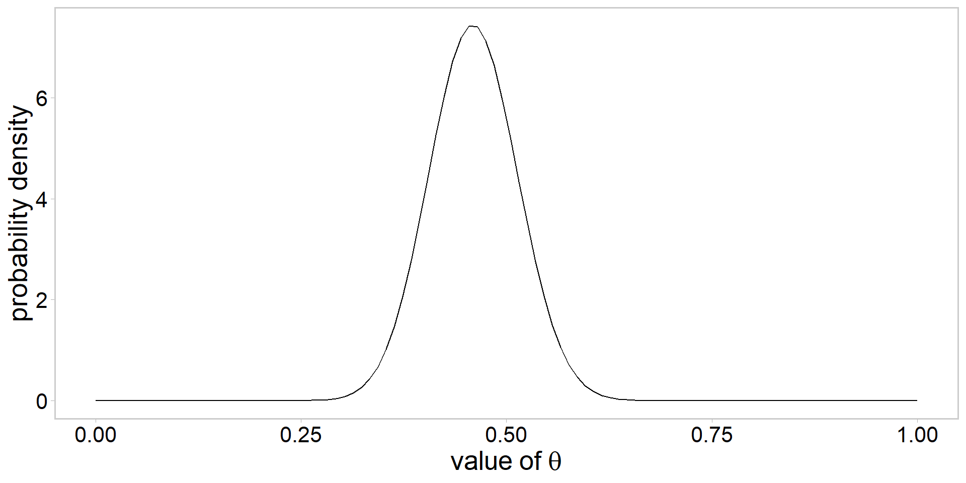
Plot the unstandardized log-posterior
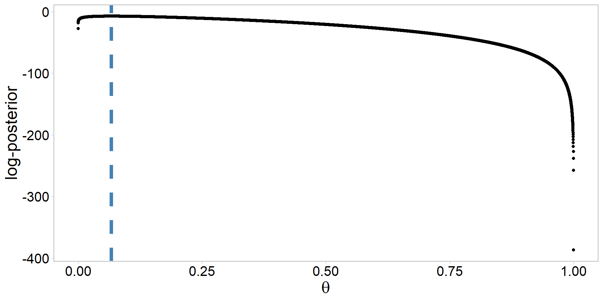
Plot the standardized posterior
my_data %>%
  ggplot(aes(x = theta, y = exp(logPost) / sum(exp(logPost)))) + # note exp()
  geom_point(size = 1.4) +
  ylab("Posterior") +
  xlab(expression(theta)) +
  geom_vline(
    xintercept = MAP, linetype = 2, linewidth = 2,
    color = "steelblue"
  ) + # add MAP estimate
  theme_qfc() +
  theme(text = element_text(size = 20))