Approximating posterior distributions using simulation

FW 891
Click here to view presentation online

Christopher Cahill

30 August 2023

Recap

Last time we learned that in some special situations we could generate analytical posterior distributions (e.g., the beta-binomial model)
However, the reality is that this only works for simple models (i.e., typically < 3 parameters)
Today we explore a broad class of computational methods and algorithms aimed at approximating posterior distributions
We will still use simple models today, but realize that some of these tools scale far better than others to high-dimensional space

Outline

Computing a posterior via grid approximation
Markov Chain Monte Carlo
Metropolis-Hastings algorithm
Hamiltonian Monte Carlo

Grid search approximation: the basics

Recall that: \[ \color{darkgreen}{posterior} \propto \color{#E78021}{likelihood} \cdot \color{#3697DC}{prior} \]
For models with 1-2 parameters approximating the posterior is actually a fairly tractable problem, even when the math isn’t nice
All we do is create a “grid” of parameter values and compute the posterior
We then search across the computed posterior values to find the posterior maximum and corresponding parameter estimates

Revisiting the sneak turtles with different priors

library(tidyverse)
library(ggqfc)
y <- c(
  0, 0, 0, 0, 0, 0, 0, 0, 1, 0, 0, 0, 0, 1, 0,
  0, 0, 0, 0, 0, 0, 0, 0, 0, 0, 0, 0, 0, 0, 0
) # sucesses (turtle detections)
n <- length(y) # trials

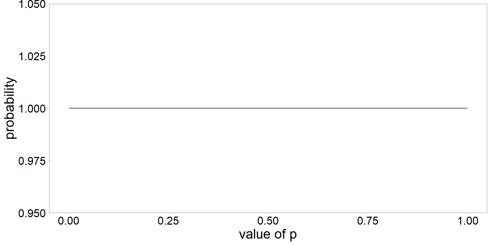
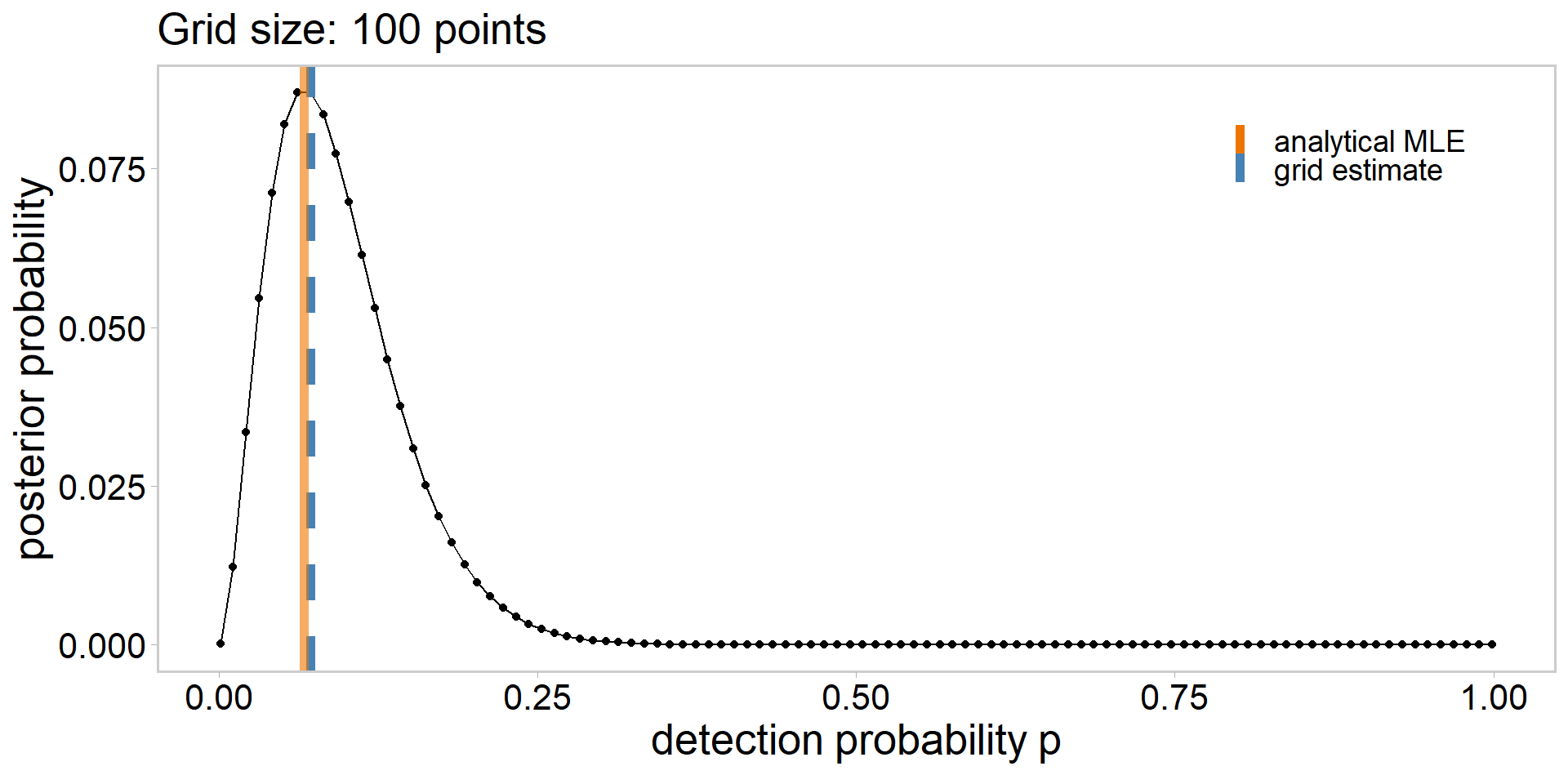
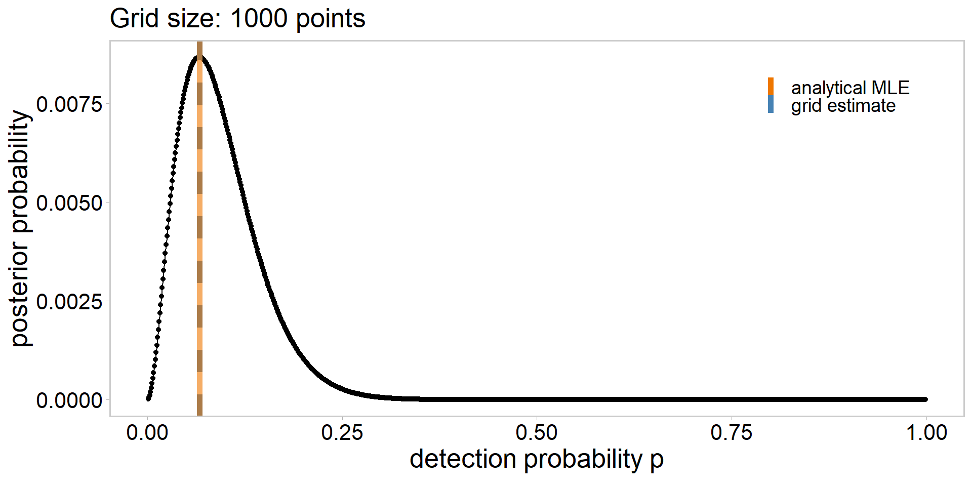
# define a grid
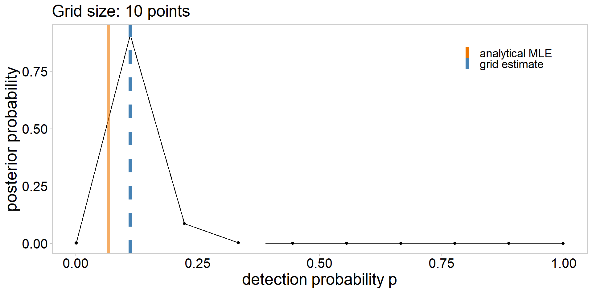
grid_size <- 10
p_grid <- seq(from = 1e-3, to = 0.999, length.out = grid_size)

# calculate likelihood
lik <- dbinom(sum(y), n, p_grid)
lik # likelihood of having observed the data | each p_grid value

 [1] 4.229830e-04 1.964028e-01 1.859940e-02 5.603740e-04 6.085257e-06
 [6] 1.860800e-08 8.682232e-12 1.445413e-16 7.970008e-25 4.341304e-82

see ?dunif, ?dnorm, ?dbinom, etc.

Always work in log-space when dealing with likelihoods and prior probabilities!

Recognize that \[ \color{darkgreen}{posterior} \propto \color{#E78021}{likelihood} \cdot \color{#3697DC}{prior} \]

is the same as \[ \color{darkgreen}{log(posterior)} \propto \color{#E78021}{log(likelihood)} + \color{#3697DC}{log(prior)} \]

When we multiply likelihoods together they get smaller and may surpass machine precision, so we usually work in log-space

Back to the R side of things…

# Note that
log(lik)

 [1]   -7.768179   -1.627588   -3.984626   -7.486906  -12.009642  -17.799674
 [7]  -25.469743  -36.472966  -55.488942 -187.343803

# is the same as
log_lik <- dbinom(sum(y), n, p_grid, TRUE)
log_lik

 [1]   -7.768179   -1.627588   -3.984626   -7.486906  -12.009642  -17.799674
 [7]  -25.469743  -36.472966  -55.488942 -187.343803

We have now defined the log-likelihood across our entire grid sequence of \(p\)
Now we need to calculate the prior probabilities at each p_grid value

Dealing with the prior probablities

Assume \(p\sim \mathrm{Uniform}(0, 1)\)
We can calculate the log(prior probability) for each \(p\) in our grid given a uniform prior via:

log_prior <- dunif(p_grid, 0, 1, TRUE)
log_prior

 [1] 0 0 0 0 0 0 0 0 0 0

Is this correct?

Visualizing the Uniform prior

Calculating the posterior

Now can calculate the posterior probabilities of each p_grid value given the likelihood and prior as follows:

# unstandardized log posterior
log_unstd_post <- log_lik + log_prior

# exponentiate the log posterior
unstd_post <- exp(log_unstd_post)

# standardize it (so probabilities sum to one)
post_prob <- unstd_post / sum(unstd_post)

# Put everything together in a data frame
posterior <- data.frame(
  p = p_grid, log_lik, log_prior,
  log_unstd_post, post_prob
)

Let’s take a look at our posterior approximation

posterior

           p     log_lik log_prior log_unstd_post    post_prob
1  0.0010000   -7.768179         0      -7.768179 1.958330e-03
2  0.1118889   -1.627588         0      -1.627588 9.093073e-01
3  0.2227778   -3.984626         0      -3.984626 8.611164e-02
4  0.3336667   -7.486906         0      -7.486906 2.594424e-03
5  0.4445556  -12.009642         0     -12.009642 2.817357e-05
6  0.5554444  -17.799674         0     -17.799674 8.615147e-08
7  0.6663333  -25.469743         0     -25.469743 4.019707e-11
8  0.7772222  -36.472966         0     -36.472966 6.691985e-16
9  0.8881111  -55.488942         0     -55.488942 3.689961e-24
10 0.9990000 -187.343803         0    -187.343803 2.009941e-81

which.max(posterior$post_prob)

[1] 2

posterior[which.max(posterior$post_prob), ] # best estimate of p

          p   log_lik log_prior log_unstd_post post_prob
2 0.1118889 -1.627588         0      -1.627588 0.9093073

Key points:

For each value of \(p\) in p_grid we get

log-likelihood of the data | that \(p\)
log-prior probability for that \(p\) | the prior(s)
log-posterior calculation for each \(p\) (very much not a probability)
posterior probability for each \(p\)

Key points continued:

The log-likelihood refers to the joint density of all data points (i.e., the sum of the log-likelihood values for each datum)
log-prior is the marginal distribution of the parameter(s)

Comparing our grid approximation with the analytical MLE

Exercise

A new study estimated the detection probability of sneak turtles, and you want to incorporate this information as prior information into your analysis
Repeat the analysis above in R with a grid_size of 10000 and a \(p\sim \mathrm{Normal}(0.13, 0.12)\)
Report your best estimate of log-posterior and p given this prior
If you get this far, try a bunch of different normal priors and think about how it influences your findings

Solution

             p   log_lik log_prior log_unstd_post    post_prob
747 0.07545825 -1.289803  1.098033     -0.1917702 0.0008715062

Why can’t we just grid search everything?

There are many important model types (e.g., mixed effects models) for which analytical solutions and things like grid appoximation fail miserably
- For models with many parameters and a dense grid, computational burden is intractable
- This includes almost all models relevant to applied ecology

The Bayesian problem

\[ P(\theta \mid y)=\frac{P(y \mid \theta) P(\theta)}{P(y)} \]

\(P(y)\) is called the “evidence” (i.e. the evidence that the data y was generated by this model)
We can compute this quantity by integrating over all possible parameter values:

\[ P(y)=\int_{\Theta} P(y, \theta) \mathrm{d} \theta \]

The Bayesian problem cont’d

This is the key difficulty with Bayesian statistics, and is why Bayesian statistics was not popular until computing power increased in the 1990s
- Even for relatively simple models this thing can be intractable
If we can’t solve it, can we approximate it via Monte Carlo?
- Monte Carlo = repeated random sampling
Unfortunately this would require us to first solve Bayes’ theorem because we don’t know what the distribution \(P(\theta \mid y)\) is

McElreath 2023 chapter 2

The Bayesian problem cont’d

So we can’t compute it using standard methods, can’t sample directly from it
Mathematicians realized this, and instead said:
- “Let’s construct an ergodic, reversible Markov chain that has as an equilibrium distribution which matches our posterior distribution”
What? 🦇💩
Markov chain: what happens next depends only on the state of affairs now
The remarkable fact is that this is relatively easy to do Gelman et al. 2003

Introduction to Markov Chain Monte Carlo (MCMC)

What is MCMC: a broad class of algorithms that allow us to sample from an arbitrary probability distribution
Counter-intuitive to most non-robots
Rather than computing the \(P(\theta \mid y)\) directly, MCMC draws samples of parameters from \(P(\theta \mid y)\)
- This is actually extremely useful
Collecting enough samples allows us to ‘map out’ or get a picture of \(P(\theta \mid y)\)

The Metropolis-Hastings algorithm

Metropolis–Hastings (MH) is a classic MCMC algorithm with the following rules:
Let \(f(x)\) be a function that is proportional to the desired probability density function \(P(x)\) (a.k.a the “target distribution”)
Remember that we know:

\[ \color{darkgreen}{posterior} \propto \color{#E78021}{likelihood} \cdot \color{#3697DC}{prior} \]

So we just set \(f(x)\) = \(P(y \mid \theta) \cdot P(\theta)\)

The Metropolis-Hastings algorithm cont’d

The recipe:

Choose an arbitrary starting value for a parameter \(x_{t}\)
Choose an arbitrary probability distribution \(g(x \mid y)\) to propose the next parameter value \(x\) given the previous value \(y\)
- Note \(g(x \mid y)\) is usually a Gaussian distribution centered at \(y\) so that points closer to \(y\) are more likely to be visited next (random walk)

Gelman et al. 2003

The Metropolis-Hastings algorithm cont’d

for each iteration \(t\)
- generate a proposed value for \(x^{\prime}\) by drawing a random number from \(g\left(x^{\prime} \mid x_{t}\right)\)
- calculate the acceptance probability (a.k.a. acceptance ratio) \(\alpha=f\left(x^{\prime}\right) / f\left(x_{t}\right)\)
- accept or reject the proposed value \(x^{\prime}\)
  - generate a uniform random number \(u \in[0,1]\)
  - if u > \(\alpha\), accept the proposal and set \(x_{+1}=x^{\prime}\)
  - if u < \(\alpha\), reject the proposal and set \(x_{+1}=x_{t}\)

Gelman et al. 2003

Re-thinking the acceptance probability

This thing works because

\(\alpha=f\left(x^{\prime}\right) / f\left(x_{t}\right)\)

is the same as saying

\[ \alpha=\frac{\frac{P(y \mid \theta^{\prime}) P(\theta^{\prime})}{P(y)}}{\frac{P(y \mid \theta_{t}) P(\theta_{t})}{P(y)}} \]

Note we just substituted \(x^{\prime}\) and \(x_{t}\) for \(\theta^{\prime}\) and \(\theta_{t}\)

\(P(y)\) cancels out via mathemagicks

Remember the sneak turtles 🐢!

 [1] 0 0 0 0 0 0 0 0 1 0 0 0 0 1 0 0 0 0 0 0 0 0 0 0 0 0 0 0 0 0

[1] 30

Building a Metropolis-Hastings algorithm for sneak turtles 🐢

First, write three helper functions:

l_prior <- function(param) { # log(prior)
  dunif(param, min = 0, max = 1, log = T) # uniform(0,1) prior
}

l_lik <- function(param) { # log(likelihood)
  dbinom(sum(y), n, param, log = T)
}

l_post <- function(param) { # log(posterior) = log(likelihood) + log(prior)
  l_lik(param) + l_prior(param)
}

Building a Metropolis-Hastings algorithm for sneak turtles 🐢

Second, declare some stuff

n_iter <- 10000 # number of iterations to run the MCMC
chain <- rep(NA, n_iter) # place to store values of p
chain[1] <- 0.5 # initial guess at p

Building a Metropolis-Hastings algorithm for sneak turtles 🐢

Now we run the algorithm

for (i in 2:n_iter) {
  p_new <- rnorm(1, chain[i - 1], 0.1) # new proposed p based on previous p

  # next two lines ensure new p stays between [0,1] - ignore them
  if (p_new < 0) p_new <- abs(p_new)
  if (p_new > 1) p_new <- 2 - p_new

  a_prob <- exp(l_post(p_new) - l_post(chain[i - 1])) # acceptance prob

  if (runif(1) < a_prob) {
    chain[i] <- p_new # accept the proposal
  } else {
    chain[i] <- chain[i - 1] # reject the proposal
  }
}

see also Gelman et al. 2003; Robert and Casella 2010

Metropolis-Hastings results

Exercise

Get in groups of three, play with the following:

the proposal distribution
the initialization value
chain length
plot histogram of p and the chain (the fuzzy catepillar plot)

Report your findings back to the group

MCMC algorithm diagnostics

Many of the parameters we were playing with affect our approximation of the posterior!
Remember, this is a dead-simple example. Eventually we will use MCMC to approximate high-dimensional integrals which is much more difficult
Clearly takes some time to “converge” on a stable posterior distribution
- With MH MCMC this period between initial values and convergence to some distribution is known as the “burn-in” period, and we usually discard it

Gelman et al. 2003; Kery and Schaub 2013; McElreath et al. 2023

Proposal distribution sd = 0.001

Proposal distribution sd = 0.002

Proposal distribution sd = 0.005

Proposal distribution sd = 0.01

Proposal distribution sd = 0.1

Proposal distribution sd = 0.2

Proposal distribution sd = 0.4

Proposal distribution sd = 0.42

Proposal distribution sd = 0.44

Proposal distribution sd > 0.44

Breaks the following lines and dies because gives p outside [0,1]

if (p_new < 0) p_new <- abs(p_new)
if (p_new > 1) p_new <- 2 - p_new

There are smarter ways to keep a value between [0,1]
Key points:
- tuning the algorithm impacts its ability to sample the posterior
- correlation in the Markov chain means you don’t get independent samples of the parameters of interest

What do we want the chains to do

We want chains to look like fuzzy caterpillars

Good indication that the MCMC is efficiently sampling from a maximum in the underlying distribution

Fuzzy caterpillars are good indication that a chain is behaving, but…

We could be stuck in a local maximum
- If we ran it longer we might find a better solution
- One way to deal: run multiple, independent chains initialized from different starting locations
Should get overlapping fuzzy caterpillars if everything goes well
Because chains are independent, we often run them in parallel

Gelman et al. 2003; Kery and Schaub 2013; McElreath et al. 2023

Running multiple chains each with different initialization values

Software that can run MCMC for you

BUGS/JAGS
NIMBLE (de Valpine et al. 2017)
MCMCpack
LaplacesDemon
Stan (what we will use in this class)
Many others

These tools implement many different MCMC routines Ecologists can (mostly) treat these tools as black boxes

e.g., see Gelman et al. 2003; Green et al. 2020; Kery and Schaub 2013

Hamiltonian Monte Carlo (HMC)

The following draws heavily from Chapter 9 in McElreath 2023

It appears to be a quite general principle that, wherever there is a randomized way of doing something, then there is a nonrandomized way that delivers better performance but requires more thought-E.T. Jaynes

No free lunch

Wikipedia

Hamiltonian Monte Carlo (HMC)

HMC is much more computationally demanding than MH, but its proposals are much more efficient
HMC requires fewer samples to map out the posterior distribution

The bottom line:
You need less computer time in total, even though each sample requires more time than simpler algorithms

Really outshines other algorithms for models with 10s to 1000s of parameters
Don’t need to know everything (lots of math in references)

see McElreath 2023 chapter 9

HMC: understanding some concepts

Leverages tools from Hamiltonian dynamics and differential geometry to generate better proposals
Uses information on the gradient (curvature) of the log-posterior
HMC creates a \(\theta^{\prime}\) that is uncorrelated with \(\theta_{t}\) and which has a high probability of being accepted
- Does this using a physics simulation and pretends parameters are tiny, frictionless particles
See also Neal (2011) MCMC using Hamiltonian Dynamics

HMC hockey puck analogy

Imagine you have a standard two parameter model
- This creates a posterior shaped like a bowl
In this case, HMC is like a hockey puck launched in random directions around an ice rink shaped like a bowl (the posterior distribution)

Go to MCMC interactive gallery

Stan does the HMC sneakery for you

In the Stan language, stochastic models are described by specifying stochastic or deterministic relationships between quantities such as parameters and data
Stan (software) constructs the log-posterior for you if you specify prior(s) and likelihood(s)
Applies HMC to your problem, reports chains, log-posterior, and diagnostics

Summary and outlook

Posteriors are difficult to approximate:

Analytical solutions (beta-binomial)
Brute force (grid search approximations)
MCMC (draw samples from the posterior)

We have laid the ground work, and now we get to play and fit Bayesian models in Stan

References

Gelman et al. 2003. Bayesian Data Analysis. Appendix C.
Green et al. 2020. Introduction to Bayesian Methods in Ecology and Natural Resources. Appendix B.
Kery and Schaub. 2012. Bayesian Population Analysis using WinBUGS.
McElreath 2023. Statistical Rethinking. Second Edition, Chapters 2 and 9.
Neal 2011. MCMC using Hamiltonian Dynamics. In: Handbook of Markov Chain Monte Carlo.
Robert and Casella 2010. Introduction to Monte Carlo methods with R.

Useful web link:

MCMC visualization app

Michael Betancourt seminar on using Hamiltonian Monte Carlo for Bayesian inference