library(tidyverse)
library(cmdstanr)
library(tidybayes)

set.seed(13)
n_site <- 500 # number of sampling locations for each year
# simulate random x,y site locations:
g <- data.frame(
  easting = runif(n_site, 0, 10),
  northing = runif(n_site, 0, 10)
)

locs <- unique(g)
dist_sites <- as.matrix(dist(locs)) # distances among sites
n_year <- 8 # number of yearsIntroduction to spatio-temporal models
FW 891
Click here to view presentation online
Christopher Cahill
6 November 2023
Purpose
- Goal
- Refresher on spatial random field models
- Extensions in space-time
- IID spatiotemporal random field
- random walk spatiotemporal random field
- AR(1) spatiotemporal random field
- Code demonstration for the AR(1) st model
A quick refresher
We have now seen temporal models
\[ \begin{array}{c} z_{t}= \alpha + z_{t-1}+\varepsilon_{t}, \quad \varepsilon_{t} \sim \mathrm{N}\left(0, \sigma_{p}^{2}\right), & \color{#E78021}{\text{[process equation]}} \\\\ y_{t}= z_{t}+\eta_{t}, \quad \eta_{t} \sim \mathrm{N}\left(0, \sigma_{o}^{2}\right) . & \color{#8D44AD}{\text{[observation equation]}} \\ \end{array} \]
- The time-series follows a random walk with drift or trend term \(\alpha\)
- \(\sigma_{p}^{2}\) represents process variance
- \(\sigma_{o}^{2}\) represents obsrvation variance
- \(\varepsilon_{t}\) represent process errors
- \(\eta_{t}\) represent observation errors
Auger-Methe et al. 2021
And we have also seen spatial models
\[ \begin{array}{l}\epsilon_{s} \sim \operatorname{MVN}(0, \Sigma)\\ \text{where } \Sigma \text{ is a covariance matrix with:}\\ \Sigma_{i, j}=\sigma^{2}_{gp} \exp \left( - \text {distances}_{i,j} / \theta_{gp}\right), \text { if } i \neq j \\ \Sigma_{i, j}=\sigma^{2}_{gp}, \text { if } i=j\end{array} \]
- \(\epsilon_{s}\) is a spatially explicit random effect
- \(\theta_{gp}\) controls how quickly the correlation decays between locations
- \(\sigma^{2}_{gp}\) is the marginal variability of the spatial function at all locations
- \(\text {distances}_{i,j}\) is a matrix describing Euclidean distance between sample locations
Cressie and Wikle 2011; Anderson and Ward 2019
The problem
- What if our data are indexed not only in space, but also in time?
Cressie and Wikle 2011; Anderson and Ward 2019
The problem
- What if our data are indexed not only in space, but also in time?
- We might need to account for this additional dependency in our data
Cressie and Wikle 2011; Anderson and Ward 2019
The problem
- What if our data are indexed not only in space, but also in time?
- We might need to account for this additional dependency in our data
- Why should we care about dependency?
Hurlburt 1984; Cressie and Wikle 2011; Anderson and Ward 2019
The problem
- What if our data are indexed not only in space, but also in time?
- We might need to account for this additional dependency in our data
- Why should we care about dependency?
- More generally, why go to all of this effort with spatiotemporal data?
Hurlburt 1984; Cressie and Wikle 2011; Anderson and Ward 2019
Spatiotemporal random fields
IID spatiotemporal random fields
- This is the simplest spatio-temporal random field
\[ \boldsymbol{\varepsilon}_{s,t} \sim \operatorname{MVN}\left(\mathbf{0}, \Sigma\right) \]
IID spatiotemporal random fields
- This is the simplest spatio-temporal random field
\[ \boldsymbol{\varepsilon}_{s,t} \sim \operatorname{MVN}\left(\mathbf{0}, \Sigma\right) \]
- Think of \(\boldsymbol{\varepsilon}_{s,t}\) as a matrix of sites by years
IID spatiotemporal random fields
- This is the simplest spatio-temporal random field
\[ \boldsymbol{\varepsilon}_{s,t} \sim \operatorname{MVN}\left(\mathbf{0}, \Sigma\right) \]
- Think of \(\boldsymbol{\varepsilon}_{s,t}\) as a matrix of sites by years
- The spatially correlated random effects are independent across time-steps
How do we get \(\Sigma\)?
\[ \begin{array}{l} \Sigma \text{ is a covariance matrix with:}\\ \Sigma_{i, j}=\sigma^{2}_{gp} \exp \left( - \text {distances}_{i,j} / \theta_{gp}\right), \text { if } i \neq j \\ \Sigma_{i, j}=\sigma^{2}_{gp}, \text { if } i=j\end{array} \]
How do we get \(\Sigma\)?
\[ \begin{array}{l} \Sigma \text{ is a covariance matrix with:}\\ \Sigma_{i, j}=\sigma^{2}_{gp} \exp \left( - \text {distances}_{i,j} / \theta_{gp}\right), \text { if } i \neq j \\ \Sigma_{i, j}=\sigma^{2}_{gp}, \text { if } i=j\end{array} \]
- We could also get \(\Sigma\) via other correlation kernels (Gaussian, Matern, etc.)
Let’s simulate some spatiotemporal fields in Stan
- simulate an iid spatio-temporal random field with an exponential kernel
Let’s simulate some spatiotemporal fields in Stan
- simulate an iid spatio-temporal random field with an exponential kernel
# model parameters to simulate
gp_theta <- 1 # Gaussian process scale parameter
gp_sigma <- 0.15 # Gaussian process variance / spatial noise parameter
sim_data <-
  list(
    n_sites = nrow(locs),
    n_year = n_year,
    dist_sites = dist_sites,
    gp_theta = gp_theta,
    gp_sigma = gp_sigma
  )

# compile the model
sim_mod <- cmdstan_model("week10/src/sim_st_iid.stan")
Let’s simulate a spatiotemporal field
- simulate an iid spatio-temporal random field with an exponential kernel
IID spatiotemporal random field
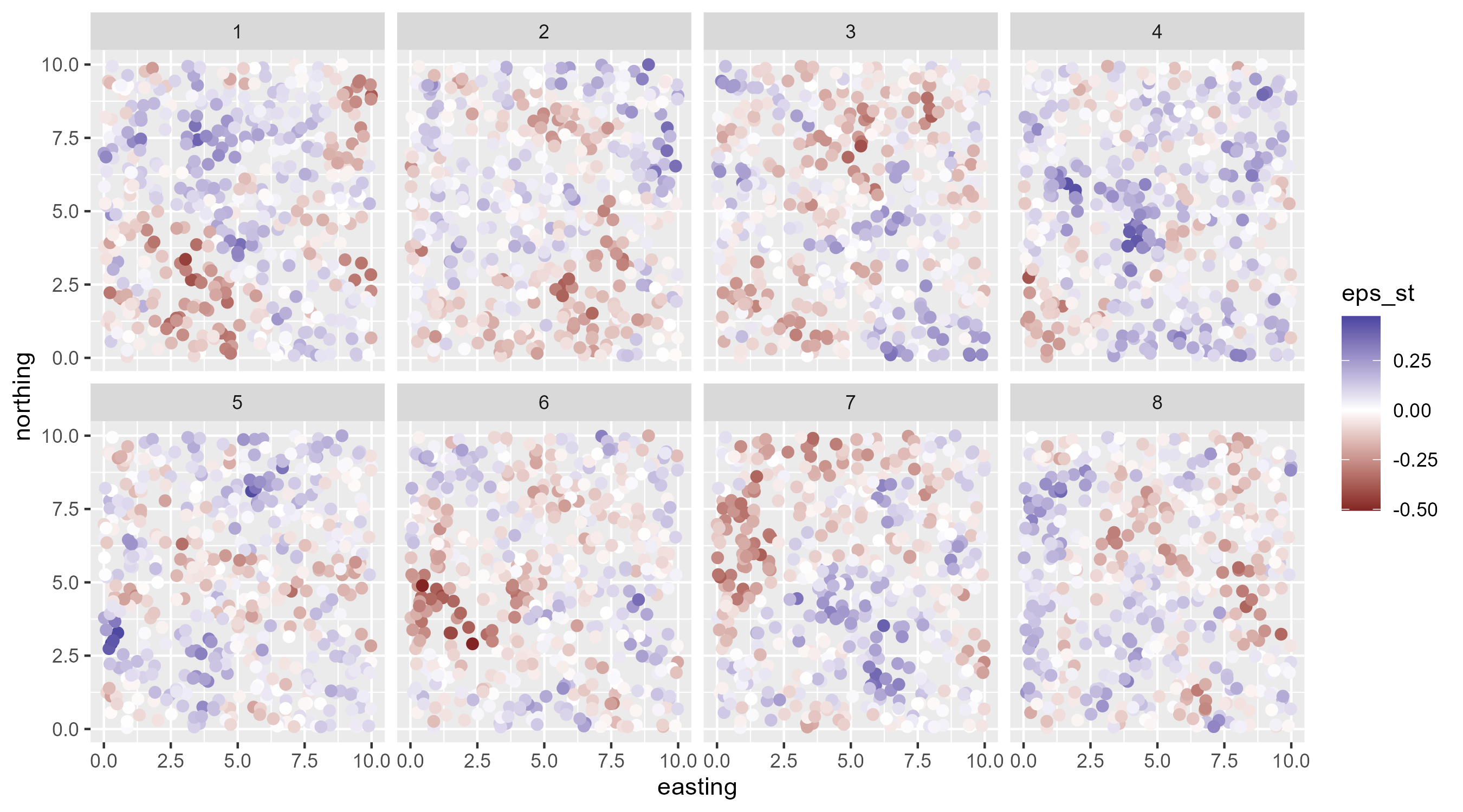
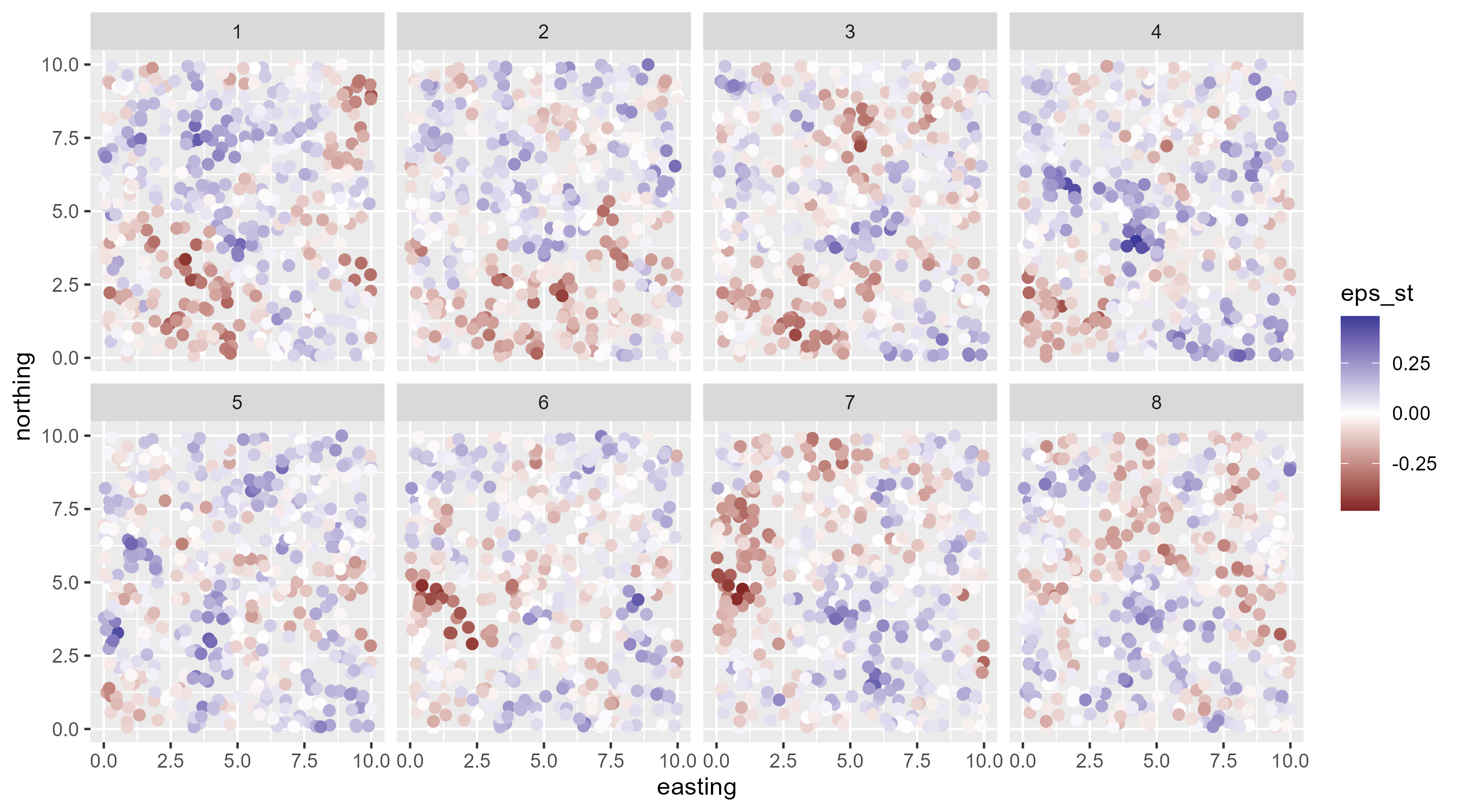
AR(1) spatiotemporal random field
AR(1) spatiotemporal random field
Autoregressive lag-1 spatiotemporal field \[ \begin{array}{l} \boldsymbol{\delta}_{t=1} \sim \operatorname{MVN}\left(\mathbf{0}, \Sigma\right) \\ \boldsymbol{\delta}_{t>1}=\rho \boldsymbol{\delta}_{t-1}+\sqrt{1-\rho^{2}} \boldsymbol{\varepsilon}_{t}, \boldsymbol{\varepsilon}_{t} \sim \operatorname{MVN}\left(\mathbf{0}, \Sigma\right), \end{array} \]
This t’s random effect is a function of previous random effect
\(\rho\) is correlation in time, must be \([-1, 1]\)
The term \(\rho \delta_{t-1}+\sqrt{1-\rho^{2}}\) scales the spatiotemporal to ensure it represents the steady-state marginal variance
AR(1) spatiotemporal random field
A random-walk (RW) spatiotemporal field
A random-walk (RW) spatiotemporal field
\[ \begin{array}{l} \boldsymbol{\varepsilon}_{s, t=1} \sim \operatorname{MVN}\left(\mathbf{0}, \Sigma\right) \\ \boldsymbol{\varepsilon}_{s,t>1} \sim \operatorname{MVN}\left(\boldsymbol{\varepsilon_{s, t-1}}, \Sigma\right), \end{array} \]
A random-walk (RW) spatiotemporal field
\[ \begin{array}{l} \boldsymbol{\varepsilon}_{s, t=1} \sim \operatorname{MVN}\left(\mathbf{0}, \Sigma\right) \\ \boldsymbol{\varepsilon}_{s,t>1} \sim \operatorname{MVN}\left(\boldsymbol{\varepsilon_{s, t-1}}, \Sigma\right), \end{array} \]
- This t’s random effect is a function of previous random effect
- No \(\rho\), which means this thing can model nonstationarity
- Note the variance is no longer steady state variance
RW spatiotemporal random field
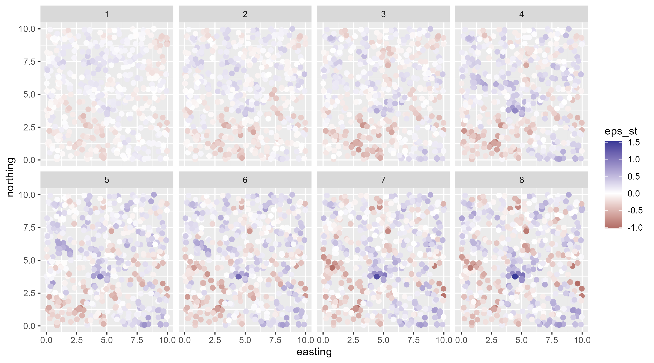
Now for a side by side of all three
IID spatiotemporal random field
AR(1) spatiotemporal random field
RW spatiotemporal random field
To the code
- Go to the Stan and R scripts
References
Anderson and Ward. 2019. Black swans in space: modeling spatiotemporal processes with extremes. Ecology.
Auger-Methe et al. 2021. A guide to state-space modeling of ecological time series. Ecological Monographs.
Cressie and Wikle 2011. Statistics for spatio-temporal data.
Hurlburt 1984. Pseudoreplication and the Design of Ecological Field Experiments. Ecological Monographs.