library(cmdstanr)# use a built in file that comes with cmdstanr:file <-file.path(cmdstan_path(), "examples","bernoulli", "bernoulli.stan")mod <-cmdstan_model(file)
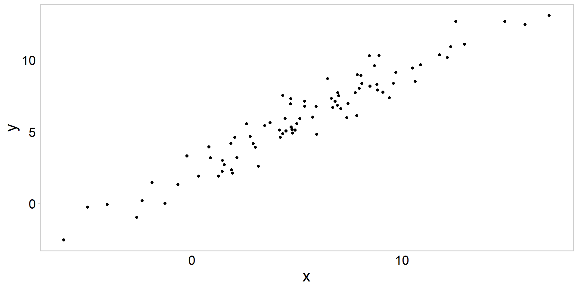
library(tidyverse)library(ggqfc)library(bayesplot)library(cmdstanr)data <-readRDS("data/linreg.rds")p <- data %>%ggplot(aes(y = y, x = x)) +geom_point() +theme_qfc() +theme(text =element_text(size =20))p
Always plot the data
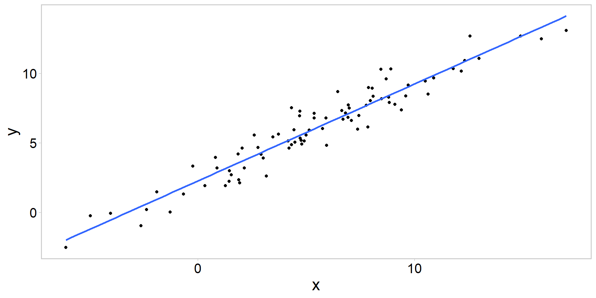
p +geom_smooth(method = lm, se = F)
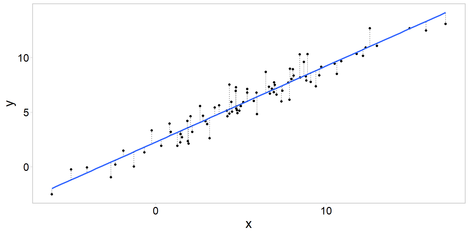
lm(data$y ~ data$x) # fit y = a + bx + e, where e ~ N(0, sd)
// this is a comment // program block demonstrationdata{// read in data here -- this section is executed one time per Stan run}transformed data {// transform the data here -- this section is also executed one time per Stan run }parameters {// declare the **estimated** parameters here }transformed parameters{ // this section takes parameter estimates and data (or transformed data) // and transforms them for use later on in model section}model{// this section specifies the prior(s) and likelihood terms, // and defines a log probability function (i.e., log posterior) of the model}generated quantities{// this section creates derived quantities based on parameters, // models, data, and (optionally) pseudo-random numbers. }
Can also write custom functions (although we won’t in this class)
In words, rather than code
As per the comments in the code, each of the program blocks does certain stuff
data{ } reads data into the .stan program
transformed data{ } runs calculations on those data (once)
parameters{ } declares the estimated parameters in a Stan program
transformed parameters{ } takes the parameters, data, and transformed data, and calculates stuff you need for your model
generated quantities{ } is only executed after you have your sampled posterior
useful for calculating derived quantities given your model, data, and parameters
Writing the linreg.stan file
data { int<lower=0> n;// number of observations vector[n] y;// vector of responses vector[n] x;// covariate x}parameters { real b0; real b1; real<lower =0> sd;}model {// priors b0 ~normal(0,10); b1 ~normal(0,10); sd ~normal(0,10);// likelihood - one way: y ~normal(b0 + b1*x, sd);// (vectorized, dropping constant, additive terms)}
Writing the linreg.stan file
data { int<lower=0> n;// number of observations vector[n] y;// vector of responses vector[n] x;// covariate x}parameters { real b0; real b1; real<lower =0> sd;}model {// priors b0 ~normal(0,10); b1 ~normal(0,10); sd ~normal(0,10);// likelihood - loopy way: for(i in1:n){ y[i] ~normal(b0 + b1*x[i], sd); }}
Writing the linreg.stan file
data { int<lower=0> n;// number of observations vector[n] y;// vector of responses vector[n] x;// covariate x}parameters { real b0; real b1; real<lower =0> sd;}model {// priors b0 ~normal(0,10); b1 ~normal(0,10); sd ~normal(0,10);// likelihood - yet another way: target +=normal_lpdf(y | b0 + b1*x, sd);// log(normal dens) (constants included)}
Key points
These three likelihood configurations result in the same parameter estimates, but option (3) will give you a different log posterior (lp__)
Vectorized option is the fastest, but sometimes these other configurations are helpful in specific applications
Stan sets up the log(posterior) as the log(likelihood) + log(priors) if you specify likelihood and priors
Some notes on priors in Stan
If you don’t specify priors, Stan will specify flat priors for you
Not always a good thing, and it can lead to problems
In this class we are either going to use vague or uninformative priors, OR we will use informative priors that incorporate domain expertise or information from previous studies
When we say a prior is “weakly informative,” what we mean is that if there’s a large amount of data, the likelihood will dominate, and the prior will not be important
Prior can often only be understood in the context of the likelihood (Gelman et al. 2017; see also prior recommendations in Stan)
see arguments in Kery and Schaub 2012; Gelman et al. 2017; McElreath 2023
Some tips for debugging .stan code
Use one chain (else prepare for impending doomies)
Use a low number of iterations (i.e., like 1-30)
wrap things in print() statements in Stan
Simulate fake data representing your model (you’ll know what truth is)
Build fast, fail fast
Plot everything
Controlling everything from linreg.R
# compile the .stan modelmod <-cmdstan_model("src/linreg.stan")# create a tagged data list# names must correspond to data block{} in .stanstan_data <-list(n =nrow(data), y = data$y, x = data$x)# write a function to set starting valuesinits <-function() {list(b0 =jitter(0, amount =0.05),b1 =jitter(0, amount =1),sd =jitter(1, amount =0.5) )}
Controlling everything from linreg.R
# what happens when we call the inits() functioninits()
Can pass this inits function to stan to initialize each of our MCMC chains at different parameter values
Running the model
fit <- mod$sample(data = stan_data, # tagged stan_data listinit = inits, # `inits()` is the function hereseed =13, # ensure simulations are reproduciblechains =4, # multiple chainsiter_warmup =1000, # how long to warm up the chainsiter_sampling =1000, # how many samples after warmpparallel_chains =4, # run them in parallel?refresh =500# print update every 500 iters)
see also ?sampling for many other options
1000 iterations for warmup and sampling is not a bad place to start (however see debugging tips at the end of the lecture)
see here for a description of runtime warnings and issues related to convergence problems
Hamiltonian based Estimated Bayesian Fraction of Missing Information (e-bfmi) quantifies how hard it is to sample level sets at each iteration
if very low (i.e., < 0.3), sampler is having a difficult time sampling the target distribution (Betancourt 2017)
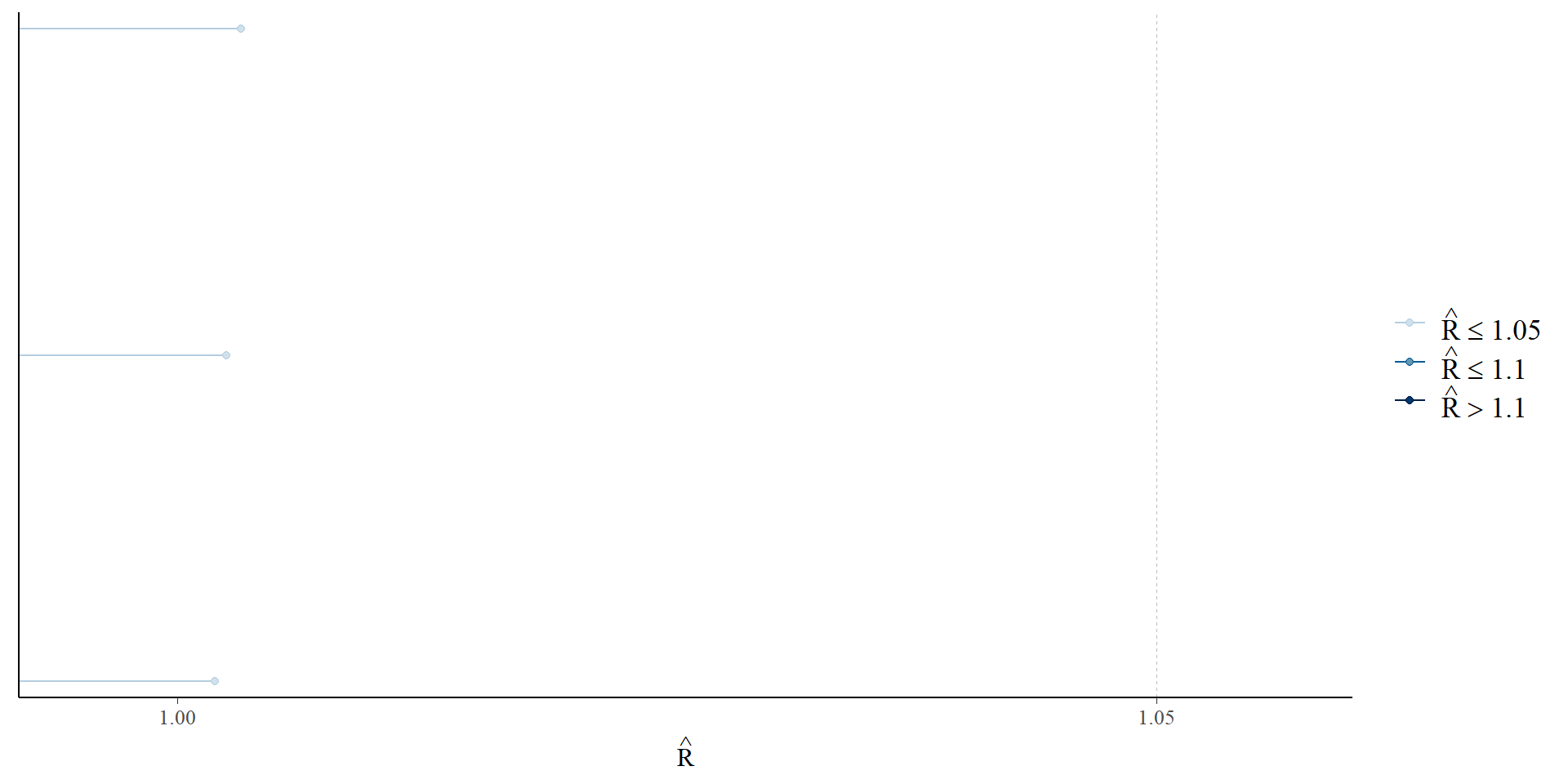
Examine \(\widehat{R}\)
# Have the chains converged to a common distribution?# compares the between- and within-chain estimates for parametersrhats <-rhat(fit)mcmc_rhat(rhats) # should all be less than 1.05 as rule of thumb
Gelman et al. 2021; McElreath 2023; Vehtari et al. 2019
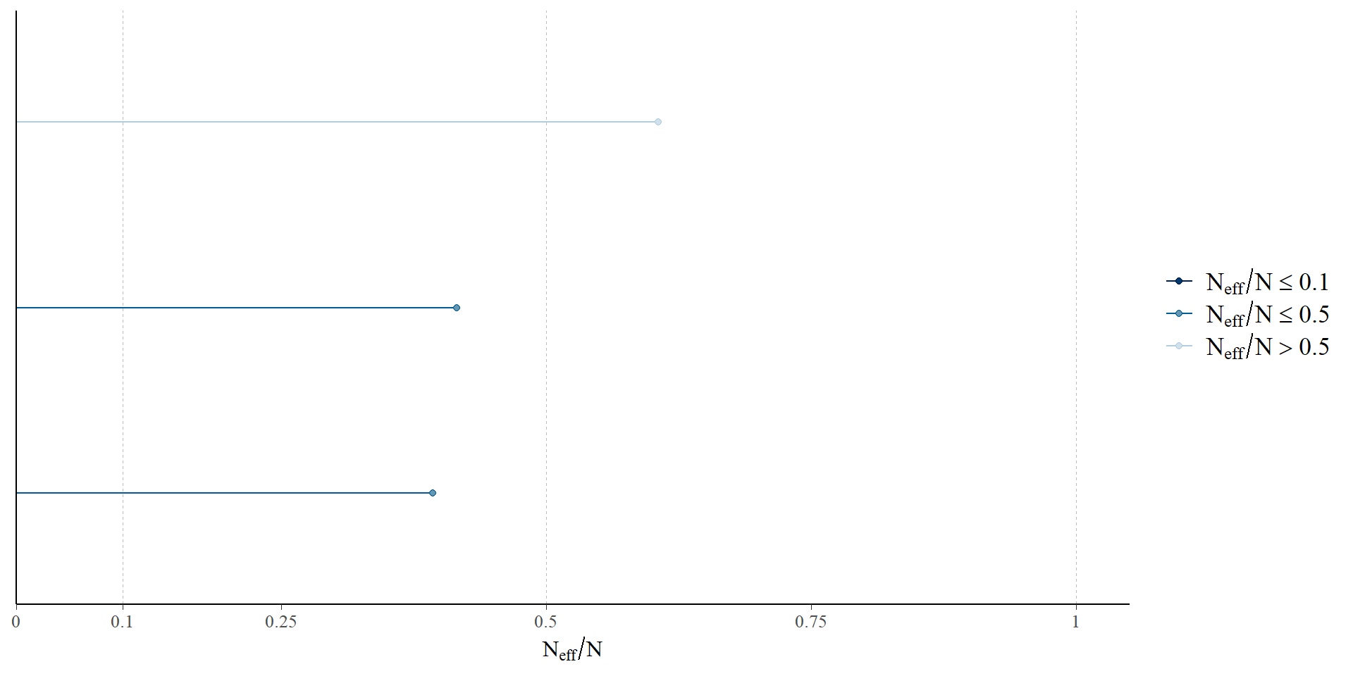
Examine the number of effective samples
eff <-neff_ratio(fit)mcmc_neff(eff) # rule of thumb is worry about ratios < 0.1
Gelman et al. 2021; McElreath 2023; Vehtari et al. 2019
Extracting the posterior draws from our CmdStanFit object
# extract the posterior drawsposterior <- fit$draws(format ="df") # extract draws x variables dfhead(posterior)
np <-nuts_params(fit) # get the sampler parameters - useful for debugging
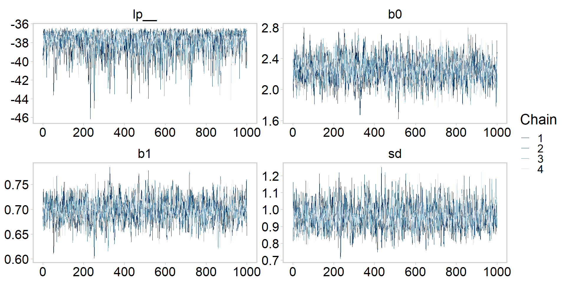
Let’s get tidy: visualizing the chains
color_scheme_set("blue") # bayesplot color themes# plot the chains of all parametersp <-mcmc_trace(posterior, np = np) +theme_qfc() +theme(text =element_text(size =20))p
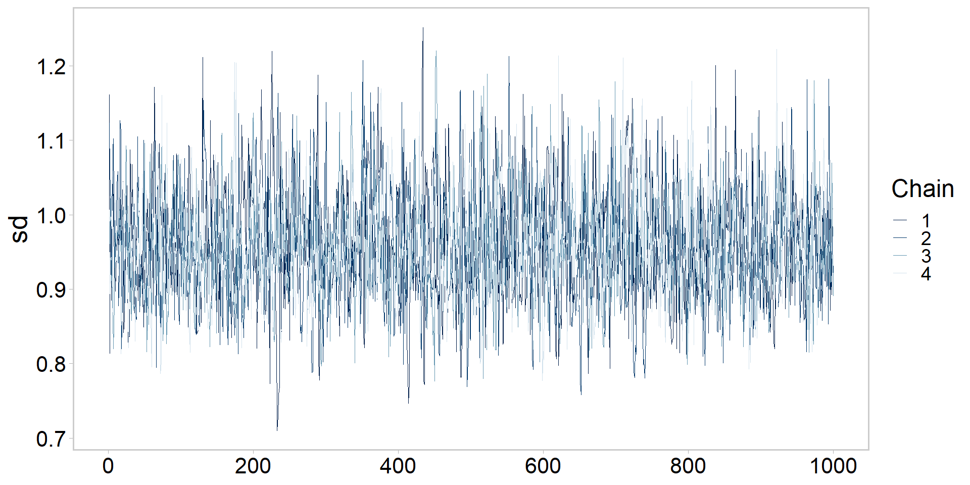
Let’s get tidy: visualizing a chain
# plot chain of one parameterp <-mcmc_trace(posterior, pars ="sd", np = np) +theme_qfc() +theme(text =element_text(size =20))p
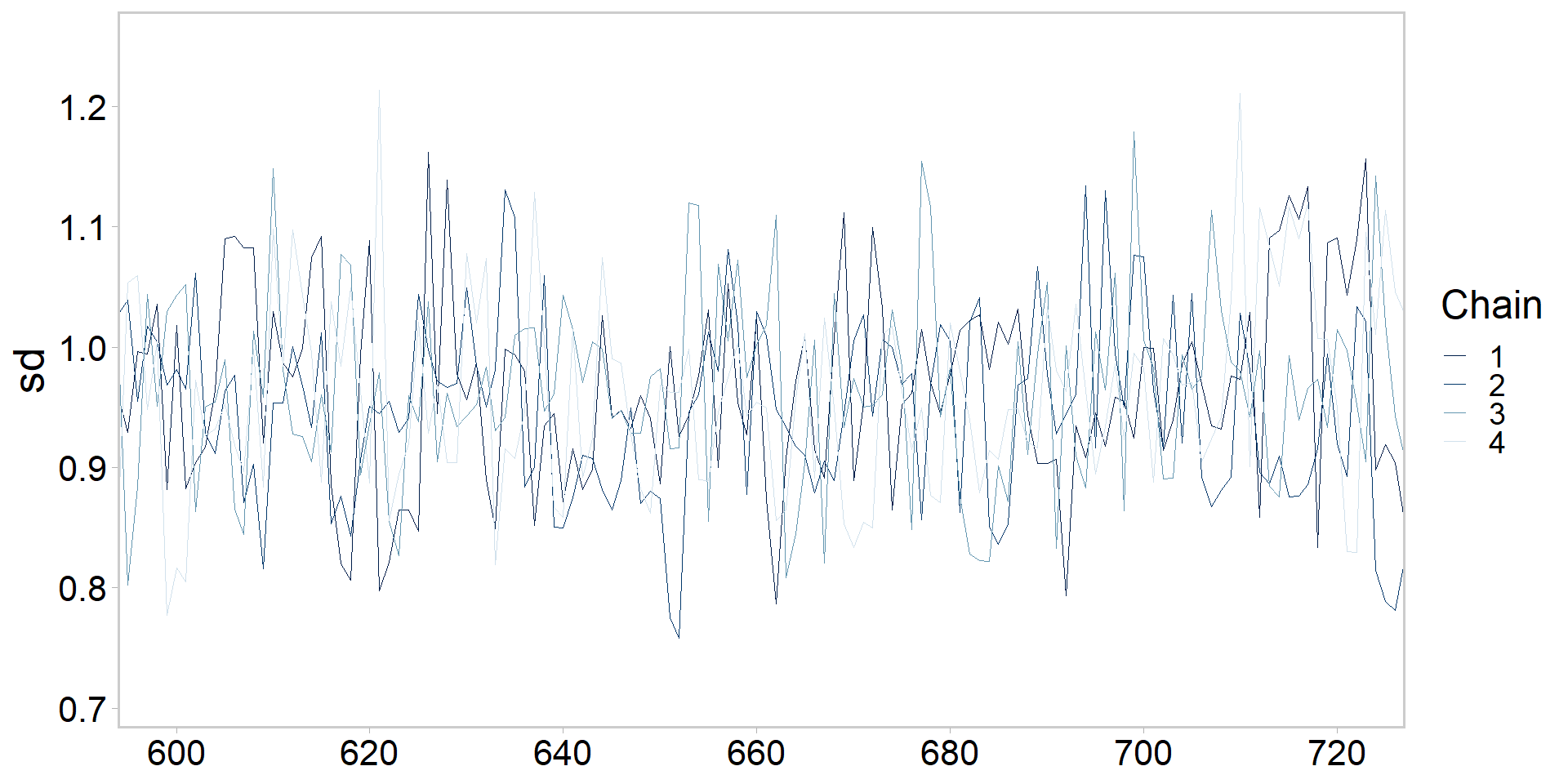
Let’s get tidy: zooming in on chains
# zoom in on one parameter iterations 600-721 (bc why not?)p <-mcmc_trace(posterior, pars ="sd", window =c(600, 721), np = np) +theme_qfc() +theme(text =element_text(size =20))p
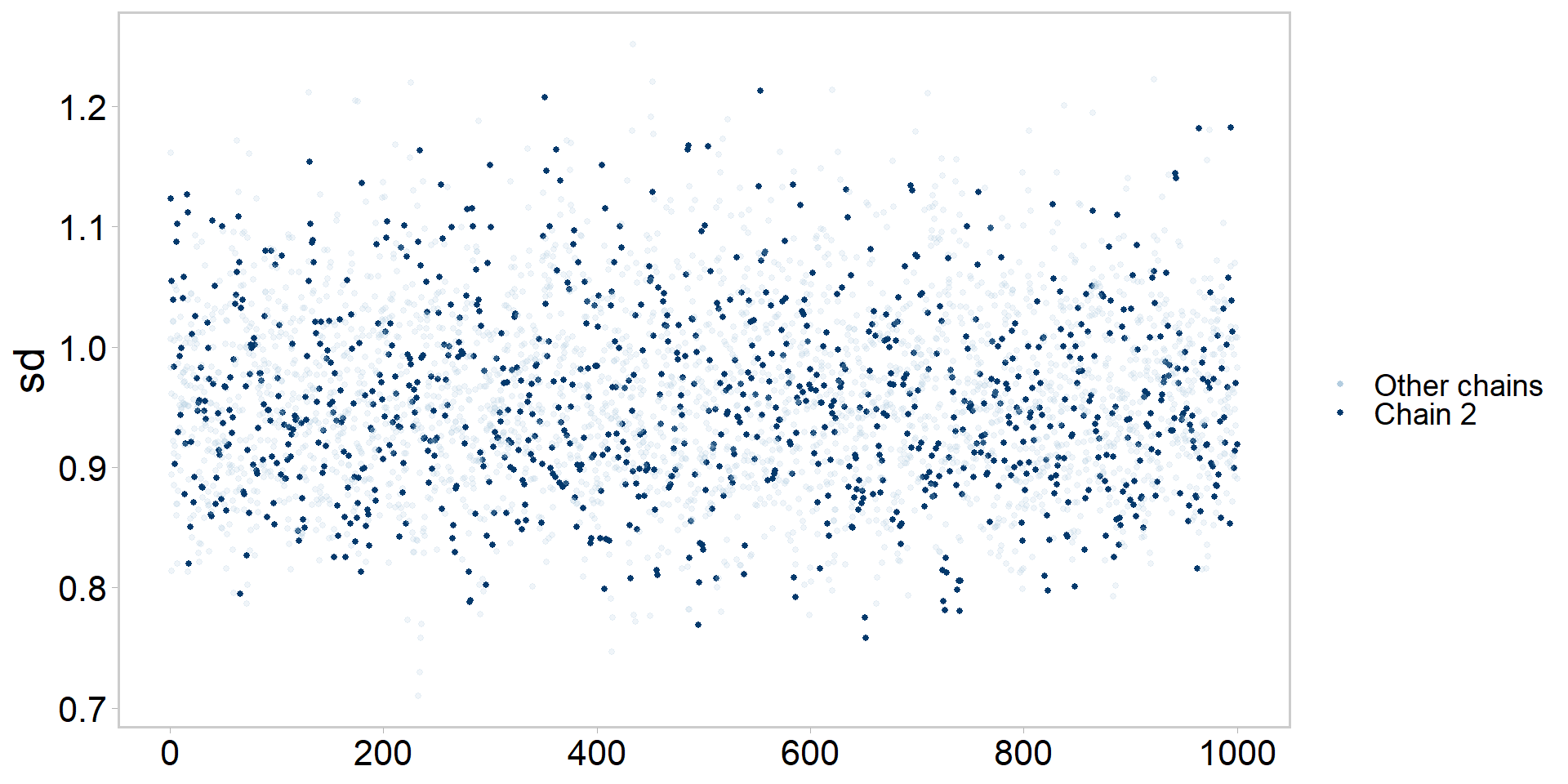
Let’s get tidy: highlighting one chain
# highlight chain 2 vs. other chains:p <-mcmc_trace_highlight(posterior, pars ="sd", highlight =2) +theme_qfc() +theme(text =element_text(size =20))p
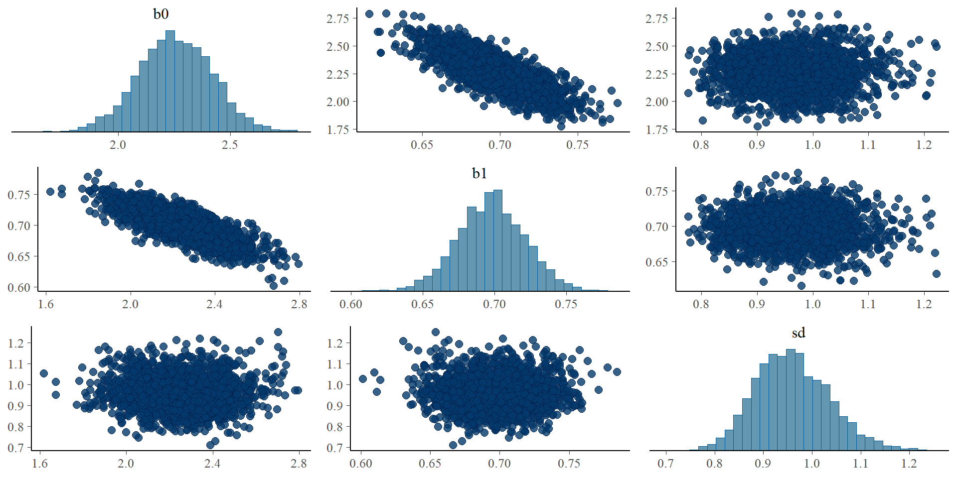
Let’s get tidy: pairs plots
# pairs plots - good modelers almost always use thisp <-mcmc_pairs(posterior, pars =c("b0", "b1", "sd"), np = np)p
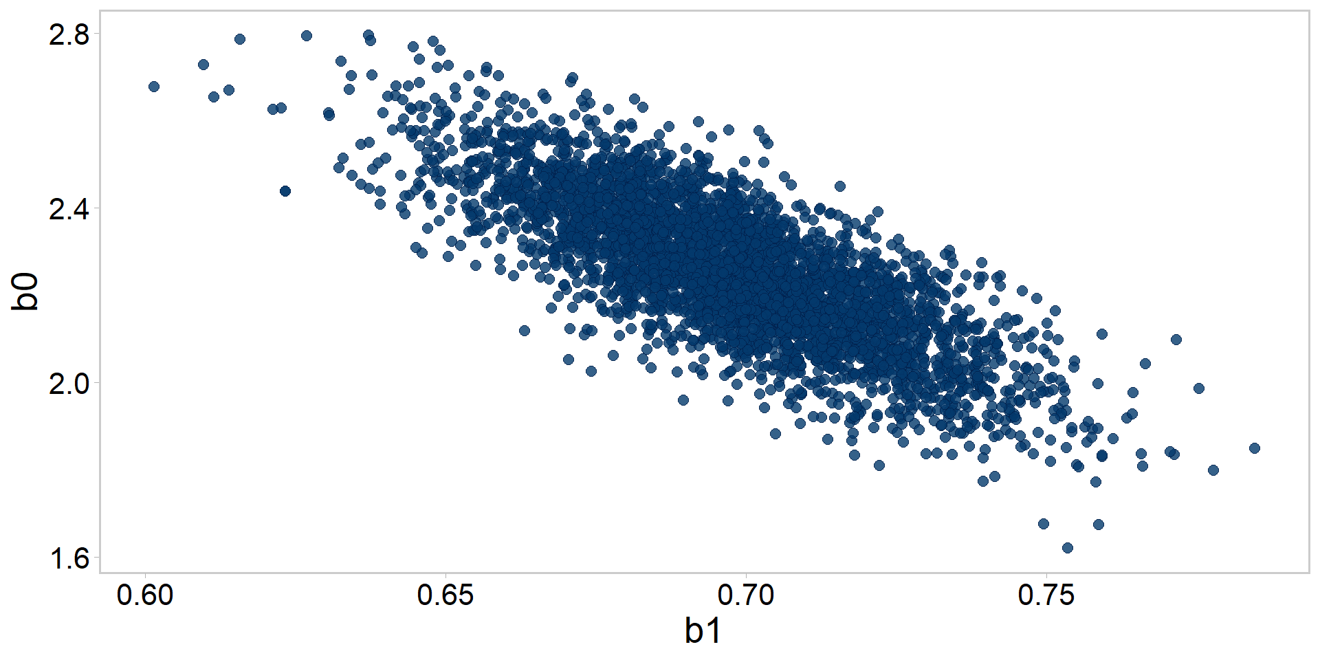
Let’s get tidy: pairs plots
# pairs plots - good modelers almost always use this# two parameters only:p <-mcmc_scatter(posterior, pars =c("b1", "b0"), np = np) +theme_qfc() +theme(text =element_text(size =20))p # check out that negative correlation!
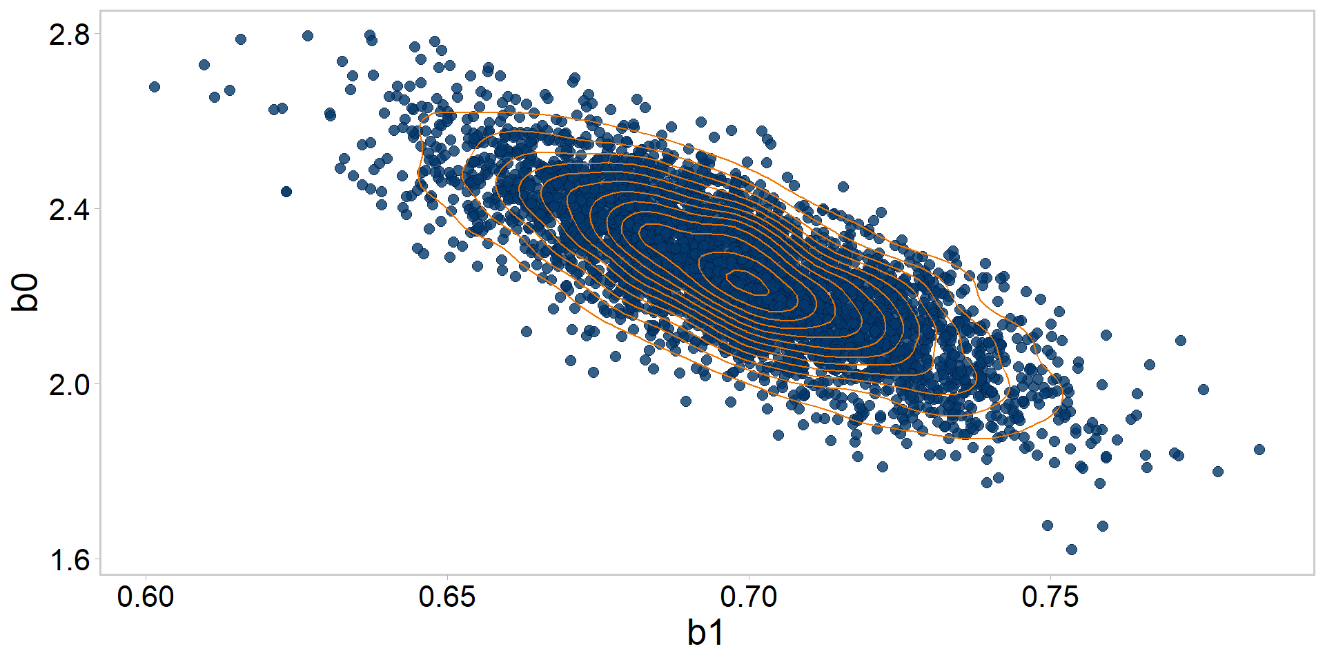
Let’s get tidy: pairs plots + quantiles
# add an 83% (why not, the world is your oyster) ellipse to itp +stat_ellipse(level =0.83, color ="darkorange2", size =1) +theme_qfc() +theme(text =element_text(size =20))
Let’s get tidy: pairs plots + contours
# visualize the posterior distribution's contours for b0, b1p +stat_density_2d(color ="darkorange2", size = .5) +theme_qfc() +theme(text =element_text(size =20))
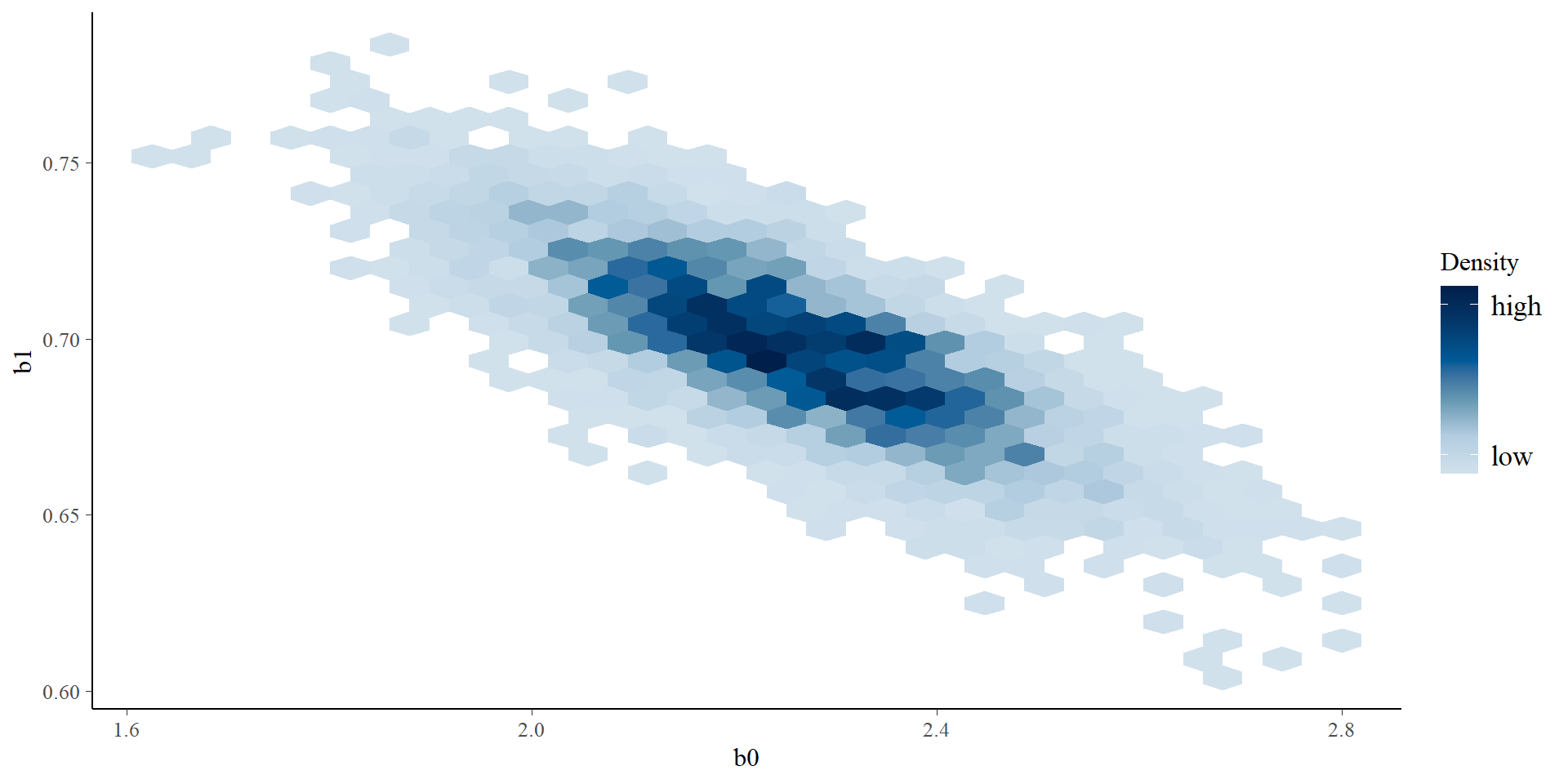
Let’s get tidy: pairs plots + contours
# view it a different waymcmc_hex(posterior, pars =c("b0", "b1"))
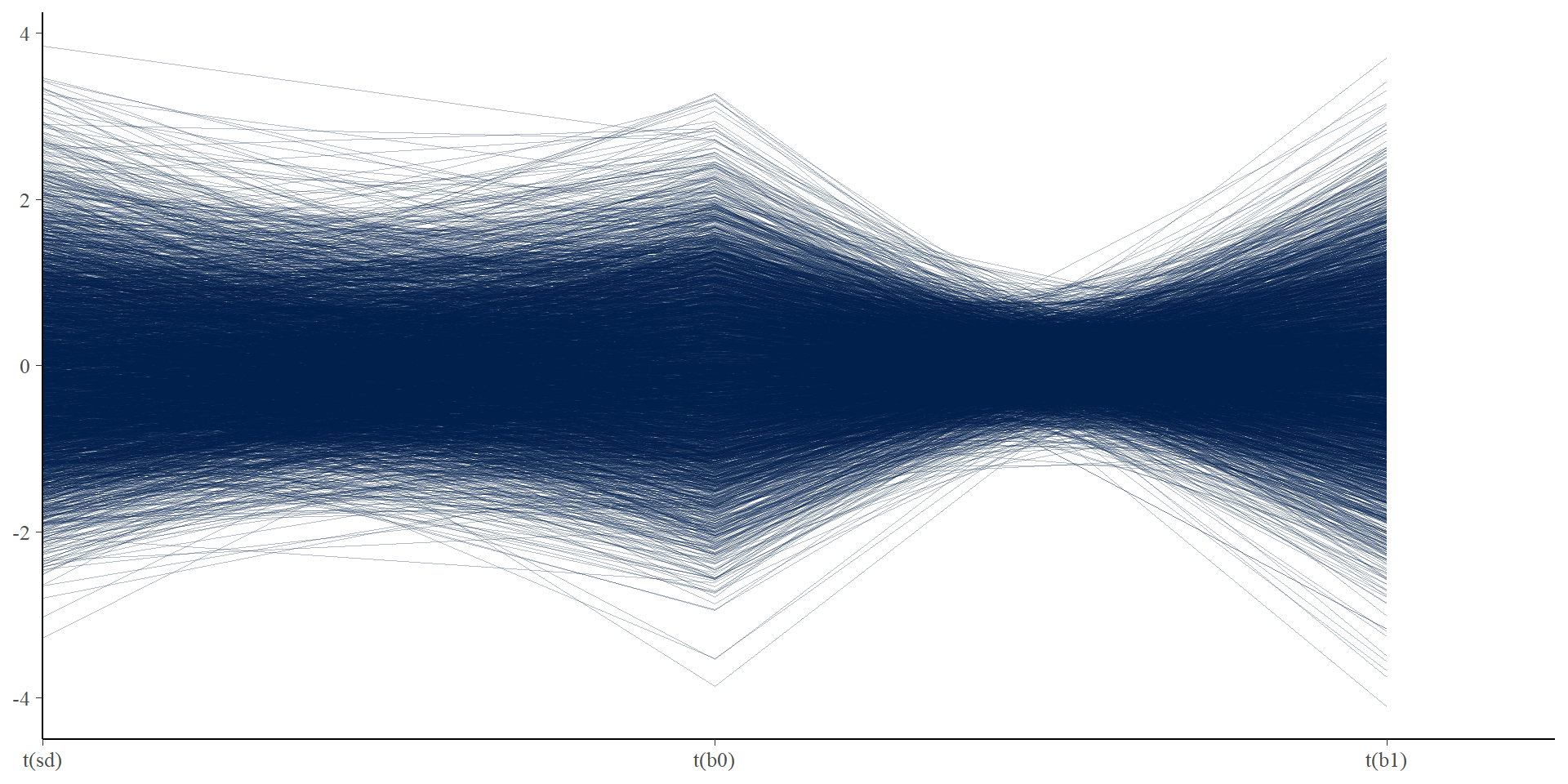
Let’s get tidy: divergent transitions
# visualizing divergent transitions# none here, but this plot shows each iteration as a line connecting# parameter values, and divergent iterations will show up as red lines# sometimes this helps you find combinations of parameters that are# leading to divergent transitionsmcmc_parcoord(posterior,pars =c("sd", "b0", "b1"),transform =function(x) { (x -mean(x)) /sd(x) # mean standardize (easier to compare) },np = np)
Let’s get tidy: divergent transitions
Moving on to fits vs. data checks
Posterior predictive checks (PPCs)
Generate replicate datasets based on our posterior draws
A great way to find discrepancies between your fitted model and the data, critical test for Bayesian models
b0 <- posterior$b0b1 <- posterior$b1sd <- posterior$sd# generate 1 dataset from the first draw of the posterior:set.seed(1)y_rep <-rnorm(length(data$x), b0[1] + b1[1] * data$x, sd[1])
Posterior predictive checks in R
# now do it for the whole posterior# loop through and create replicate datasets based on# each_draw_of_posteriorset.seed(1)y_rep <-matrix(NA, nrow =nrow(posterior), ncol =length(data$y))for (i in1:nrow(posterior)) { y_rep[i, ] <-rnorm(length(data$x), b0[i] + b1[i] * data$x, sd[i])}dim(y_rep)
[1] 4000 84
Posterior predictive checks in Stan
Can do this in Stan directly via the generated quantities{ } section:
generated quantities {// replications for the posterior predictive distributions array[n] real y_rep =normal_rng(b0 + b1*x, sd);}
Posterior predictive checks in Stan
Recompile and re-run:
mod <-cmdstan_model("src/linreg_ppc.stan")fit <- mod$sample(data = stan_data,init = inits,seed =13, # ensure simulations are reproduciblechains =4, # multiple chainsiter_warmup =1000, # how long to warm up the chainsiter_sampling =1000, # how many samples after warmpparallel_chains =4, # run them in parallel?refresh =0)
Running MCMC with 4 parallel chains...

Chain 1 finished in 0.2 seconds.
Chain 2 finished in 0.2 seconds.
Chain 3 finished in 0.2 seconds.
Chain 4 finished in 0.2 seconds.

All 4 chains finished successfully.
Mean chain execution time: 0.2 seconds.
Total execution time: 0.4 seconds.
Posterior predictive checks in Stan
Extract the posterior and take a gander at our new y_reps
posterior <- fit$draws(format ="df") # extract draws x variables data framehead(posterior)
Stan generated or simulated replicate y_rep “datasets”
n_iter*n_chain = number of posterior draws
Now compare the simulated data to our original (real) dataset
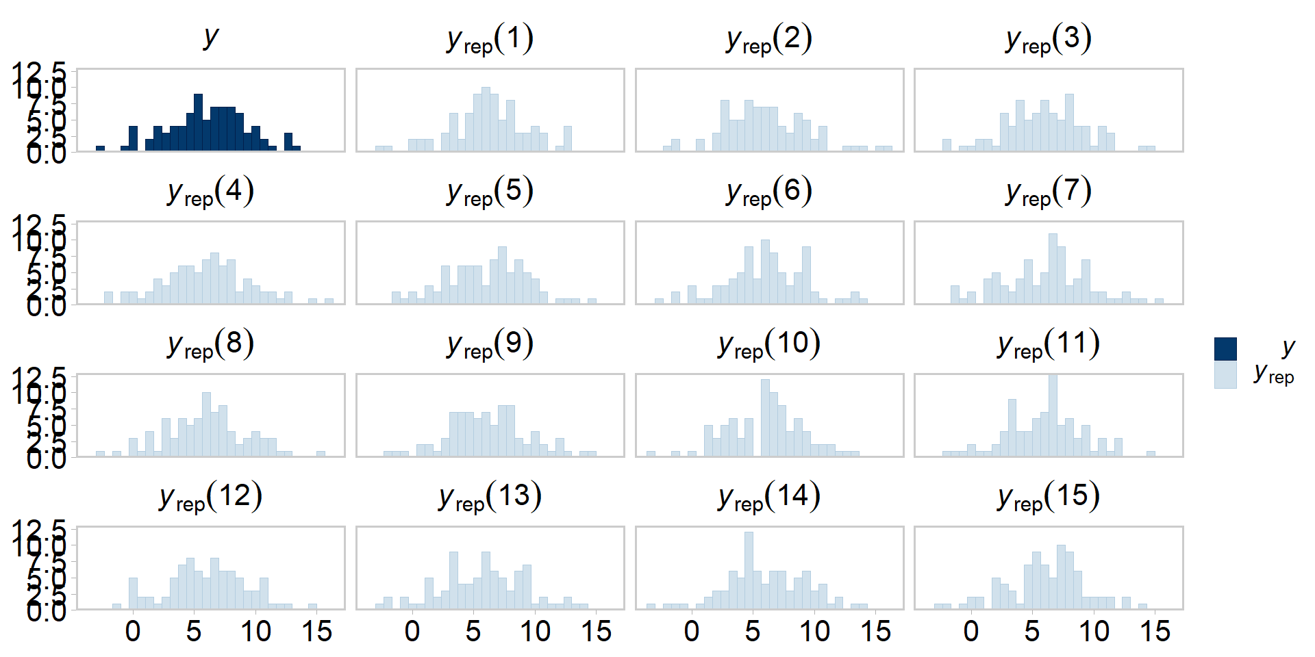
Even more tidy: visualizing PPCs
y_rep <- posterior[grepl("y_rep", names(posterior))]# compare original data against 15 simulated datasets:p <-ppc_hist(y = data$y, yrep =as.matrix(y_rep[1:15, ]))p +theme_qfc() +theme(text =element_text(size =20))
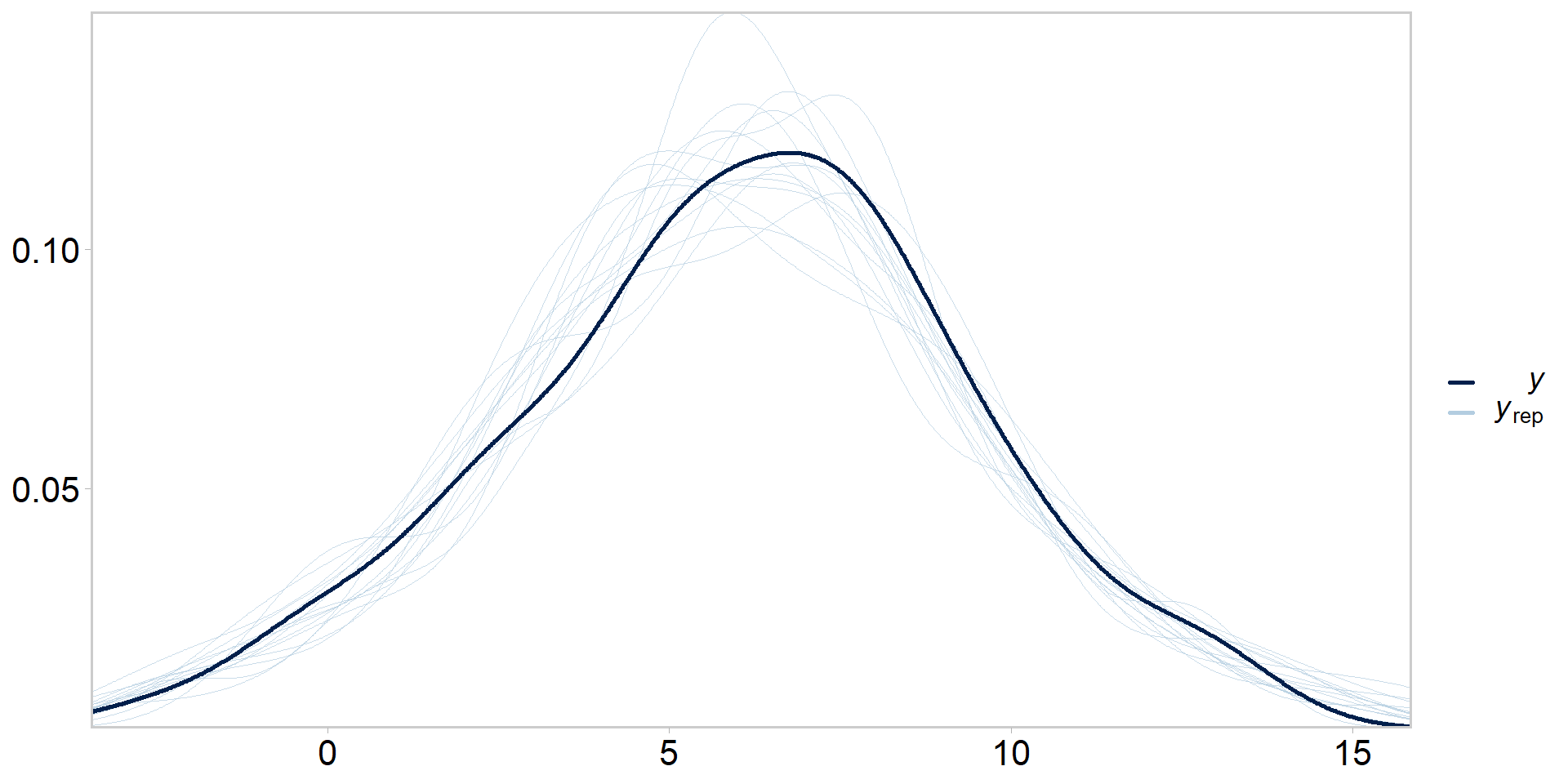
Even more tidy: visualizing PPCs
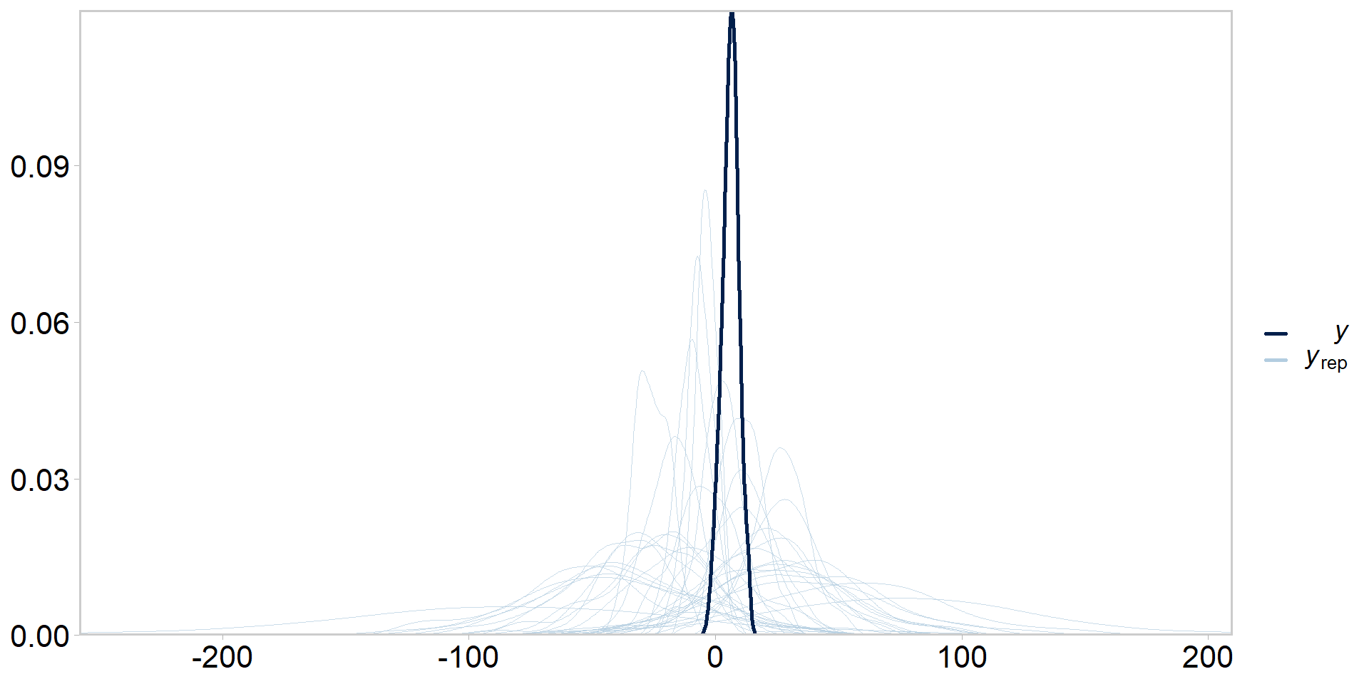
y_rep <- posterior[grepl("y_rep", names(posterior))]# compare original data against 15 simulated datasets:p <-ppc_dens_overlay(y = data$y, yrep =as.matrix(y_rep[1:15, ]))p +theme_qfc() +theme(text =element_text(size =20))
Visualizing PPCs another way
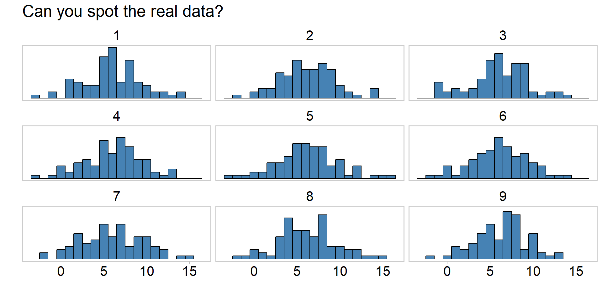
# ppcs, another wayy_reps <- y_rep[sample(nrow(y_rep), 9), ] # draw 9 replicate datsetsind <-sample(9, 1)y_reps[ind, ] <-as.list(data$y) # replace a random y_rep with true yyrep_df <- y_reps %>%as.data.frame() %>%pivot_longer(everything()) %>%# use the long format for plottingmutate(name =rep(1:9, each =ncol(y_reps)))
Visualizing PPCs another way
# ppcs, another wayyrep_df %>%ggplot() +geom_histogram(aes(x = value),fill ="steelblue",color ="black", binwidth =1 ) +facet_wrap(~name, nrow =3) +labs(x ="", y ="") +scale_y_continuous(breaks =NULL) +ggtitle("Can you spot the real data?") +theme_qfc() +theme(text =element_text(size =20))
Visualizing PPCs another way
Prior predictive checks
Same idea as posterior predictive checks, but we ignore the likelihood
Simply sample replicate datasets from the prior(s)
Tries to get at whether our priors + model configuration are consistent with our knowledge of the system
Usually would do these before posterior predictive checks, but easier to explain once you understand what posterior predictive checks are
Calculate the posterior predictive distribution one might expect for y if they went out and collected data at \(x_{i} = 1.23\)
Plot the median fit +/- 95% credible intervals from the posterior predictive distribution of y vs. \(x_{i}\). Can you think of other ways to visualize fits vs. data and the corresponding uncertainty in these fits?
Repeat the exercises in this presentation by first simulating your own linear regression dataset to prove to yourself that your code is returning reasonable answers.
Assume this dataset represents the relationship between a measure of a stream contaminant (y) and a metric of industrial development (x). Through an extensive structured decision making process it was determined by industrial representatives, resource managers, subject matter experts, and Indigenous Rightsholders that if this relationship indicated that \(\beta_{1}\) exceeded 0.71 with \(\text(Pr > 0.35)\) streamside development should be ceased. What does your analysis suggest? What are the limitations of your analysis, including things that might influence your assessment of \(\Pr(\beta_{1} > 0.71)\)? Take care to seperate explanation vs. advocacy.
Someone in the structured decision making group hates the word probability, and is pointing out that it isn’t even clear what is meant by \(\Pr(\beta_{1} > 0.71)\). Can you think of a metaphor for describing this uncertainty that does not use the word probability and which is easily understandable by folks who may lack technical training?