library(tidyverse)
library(ggqfc)
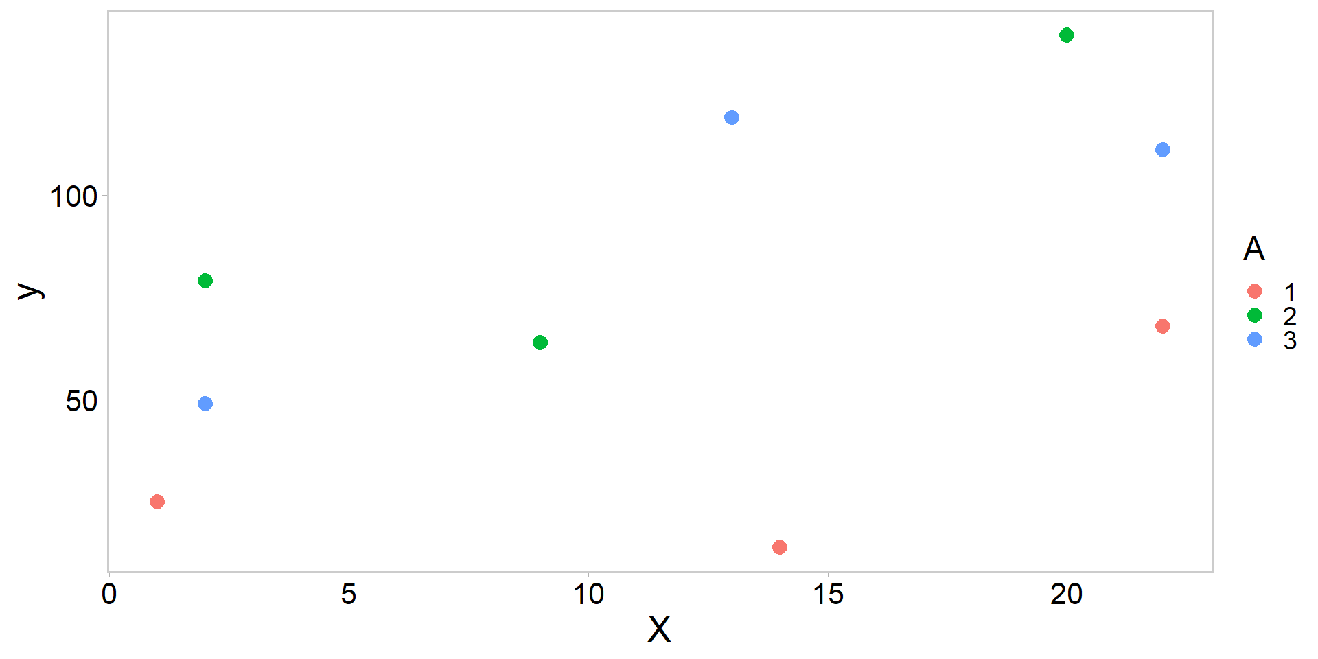
y <- c(25, 14, 68, 79, 64, 139, 49, 119, 111) # obs
A <- factor(c(1, 1, 1, 2, 2, 2, 3, 3, 3)) # group
X <- c(1, 14, 22, 2, 9, 20, 2, 13, 22) # covariate
my_df <- data.frame(y, A, X)
my_df %>%
ggplot(aes(X, y, color = A)) +
geom_point(pch = 16, size = 3.5) + theme_qfc()An introduction to Generalized Linear Models (GLMs)
FW 891
Click here to view presentation online
Christopher Cahill
11 September 2023
Purpose
- Introduce design matrices for linear models
- Introduce Generalized Linear Models
- In particular, the Poisson and binomial GLMs
- Simulate fake data from these models
- Write Stan code to estimate the parameters of these models
- A fun question
Breaking statistical models down
response = deterministic component + random component
- This section / lecture is based heavily on Kery and Schaub 2012; Kery and Royle 2016
The random (noise) component
- Hallmark of statistical models: they must account for randomness
- Check out ?ddist in R, and replace dist by any of the following: pois, binom, norm, multinom, exp, and unif
- Changing first letter d to p, q, or r allows one to get the density, the distribution function, the percentiles, and random numbers from these distributions, respectively.
- Note R calls mass functions density functions (e.g.,
dbinom())
- Note R calls mass functions density functions (e.g.,
Kery and Schaub 2012; Kery and Royle 2016
The deterministic (signal) component
- The signal component of the model contains the predictable parts of a response or the mean structure of a model
- Often the mean structure is described by a linear model, although nonlinear models can also be used (Seber and Wild 2003)
- Linear model is just one specific way to describe how we imagine our explantory variables influencing our repsonse
- This model is linear in the parameters and does not need to represent a straight line when plotted
- t-test, simple and multiple linear regressions, ANOVA, ANCOVA, and many mixed models are all linear models
Kery and Schaub 2012; Kery and Royle 2016
A brief illustration of an analysis of covariance ANCOVA
A brief illustration of an analysis of covariance ANCOVA
Running the (Frequentist) ANCOVA in R
Call:
lm(formula = y ~ A - 1 + X)

Coefficients:
    A1      A2      A3       X
1.315 65.218 58.648 2.785 - This so-called “formula language” is clever because it is quick and error-free if you know how to specify your model
- What does y ~ A−1 + X actually mean?
Kery and Schaub 2012; Kery and Royle 2016
ANCOVA maths
- When we fitted that model, we were doing the following:
\[ y_{i}=\beta_{g(i)}+\beta_{1} \cdot X_{i}+\varepsilon_{i} \quad \text {where} \quad \varepsilon_{i} \sim \operatorname{N}\left(0, \sigma^{2}\right) \]
- \(y_{i}\) is a response of unit (data point, individual, row) \(i\), \(X_{i}\) is the value of the continuous explanatory variable \(x\) for unit \(i\)
- Factor \(A\) codes for the group membership of each unit with indeces \(g\) for groups 1,2, or 3
- Two parameters in the mean relationship, \(\beta_{g(i)}\) and \(\beta_{1}\)
- First of these is a vector, second a scalar
- Index \(g\) indicates group 1, 2, or 3
ANCOVA maths: one way
\[ y_{i}=\beta_{g(i)}+\beta_{1} \cdot X_{i}+\varepsilon_{i} \quad \text {where} \quad \varepsilon_{i} \sim \operatorname{N}\left(0, \sigma^{2}\right) \]
- The random (noise) part of the model consists of the part of the response which we cannot explain using our linear combination of explanatory variables
- Represented by residuals \(\varepsilon_{i}\)
- Assume they come from a normal distribution with common variance \(\sigma^{2}\)
- How many parameters in total does this model have?
ANCOVA maths another way
Old way:
\[ y_{i}=\beta_{g(i)}+\beta_{1} \cdot X_{i}+\varepsilon_{i} \quad \text {where} \quad \varepsilon_{i} \sim \operatorname{N}\left(0, \sigma^{2}\right) \]
Shifting the structure of the model via algebra:
\[ y_{i} \sim \operatorname{N}\left(\beta_{g(i)}+\beta_{1} \cdot X_{i}, \sigma^{2}\right). \]
ANCOVA maths even more ways
A further possibility:
\[ y_{i} \sim \operatorname{N}\left(\mu_{i}, \sigma^{2}\right), \quad where \quad \mu_{i} = \beta_{g(i)}+\beta_{1} \cdot X_{i} \]
- Being able to write a linear model in algebra helps code the model in Stan (or any other modeling platform)
- Also helps you understand commonalities between many common statistical tests and what
lm()in R is doing
ANCOVA: but wait, there’s more 🥴🤔
The same model via matrix and vector notation:
\[ \left(\begin{array}{l} 25 \\ 14 \\ 68 \\ 79 \\ 64 \\ 139 \\ 49 \\ 119 \\ 111 \end{array}\right)=\left(\begin{array}{llll} 1 & 0 & 0 & 1 \\ 1 & 0 & 0 & 14 \\ 1 & 0 & 0 & 22 \\ 0 & 1 & 0 & 2 \\ 0 & 1 & 0 & 9 \\ 0 & 1 & 0 & 20 \\ 0 & 0 & 1 & 2 \\ 0 & 0 & 1 & 13 \\ 0 & 0 & 1 & 22 \end{array}\right) \times\left(\begin{array}{l} \beta_{g = 1} \\ \beta_{g = 2} \\ \beta_{g = 3} \\ \beta_{1} \end{array}\right)+\left(\begin{array}{l} \varepsilon_{1} \\ \varepsilon_{2} \\ \varepsilon_{3} \\ \varepsilon_{4} \\ \varepsilon_{5} \\ \varepsilon_{6} \\ \varepsilon_{7} \\ \varepsilon_{8} \\ \varepsilon_{9} \end{array}\right) \text {, with } \varepsilon_{i} \sim \operatorname{N}\left(0, \sigma^{2}\right) \] - Left to right: response vector, design matrix, parameter vector, residual vector
ANCOVA: but wait, there’s more 🥴🤔
The same model via matrix and vector notation:
\[ \left(\begin{array}{l} 25 \\ 14 \\ 68 \\ 79 \\ 64 \\ 139 \\ 49 \\ 119 \\ 111 \end{array}\right)=\left(\begin{array}{llll} 1 & 0 & 0 & 1 \\ 1 & 0 & 0 & 14 \\ 1 & 0 & 0 & 22 \\ 0 & 1 & 0 & 2 \\ 0 & 1 & 0 & 9 \\ 0 & 1 & 0 & 20 \\ 0 & 0 & 1 & 2 \\ 0 & 0 & 1 & 13 \\ 0 & 0 & 1 & 22 \end{array}\right) \times\left(\begin{array}{l} \beta_{g = 1} \\ \beta_{g = 2} \\ \beta_{g = 3} \\ \beta_{1} \end{array}\right)+\left(\begin{array}{l} \varepsilon_{1} \\ \varepsilon_{2} \\ \varepsilon_{3} \\ \varepsilon_{4} \\ \varepsilon_{5} \\ \varepsilon_{6} \\ \varepsilon_{7} \\ \varepsilon_{8} \\ \varepsilon_{9} \end{array}\right) \text {, with } \varepsilon_{i} \sim \operatorname{N}\left(0, \sigma^{2}\right) \]
- The value of the linear predictor for the first data point is given by \(1 \cdot \beta_{g = 1}+0 \cdot beta_{g = 2} +0 \cdot beta_{g = 3} +1 \cdot \beta_{1}\)
A trick for learning about the design matrix in R: model.matrix()
  A1 A2 A3  X
1  1  0  0  1
2  1  0  0 14
3  1  0  0 22
4  0  1  0  2
5  0  1  0  9
6  0  1  0 20
7  0  0  1  2
8  0  0  1 13
9  0  0  1 22
attr(,"assign")
[1] 1 1 1 2
attr(,"contrasts")
attr(,"contrasts")$A
[1] "contr.treatment"- see also effects or treatment contrast parameterization
model.matrix(~ A + X)
for more information on linear model see: Kery 2010
The ANCOVA in Stan
- The code looks very similar to the algebraic specification of this linear model
- Note I am picking vague-ish priors but the specific priors aren’t the point of this lesson
The ANCOVA.stan file
data {
  int<lower=0> n_obs;        // number of observations = i
  int<lower=0> n_col;        // columns of design matrix = j
  vector[n_obs] y_obs;       // observed data
  matrix[n_obs, n_col] X_ij; // design matrix: model.matrix(~A-1+X)
}
parameters {
 vector[n_col] b_j; // one parameter for each column of Xij
 real<lower=0> sig; // sigma must be postive
}
model {
  vector[n_obs] y_pred;        // container for mean response
  b_j ~ normal(0,100);         // priors for b_j
  sig ~ normal(0,100);         // prior for sig
  y_pred = X_ij * b_j;         // linear algebra sneakery
  y_obs ~ normal(y_pred, sig); // likelihood
}
And the corresponding R code:
library(cmdstanr)
mod <- cmdstan_model("week3/soln_files/ANCOVA.stan") # compile

# names in tagged list correspond to the data block in the Stan program
X_ij <- model.matrix(~ A - 1 + X)
stan_data <- list(n_obs = nrow(X_ij), n_col = ncol(X_ij),
                  y_obs = my_df$y, X_ij = as.matrix(X_ij)
                  )

# write a function to get starting values
inits <- function() {
  list(
    b_j = jitter(rep(0, ncol(X_ij)), amount = 0.5),
    sig = jitter(10, 1)
  )
}

fit <- mod$sample(
  data = stan_data,
  init = inits,
  seed = 1, # ensure simulations are reproducible
  chains = 4, # multiple chains
  iter_warmup = 1000, # how long to warm up the chains
  iter_sampling = 1000, # how many samples after warmp
  parallel_chains = 4 # run them in parallel?
)- Note this is all in the solution file for this week
Break
- Now we will move into Generalized Linear Models (GLM), where all of the information we just learned still applies
- Primary difference for GLMs is that they will allow us to model non-normal response variables in a manner similar to what we just did with an ANCOVA
- Do this via a
linkfunction
- Do this via a
Generalized Linear Models (GLMs)
- The GLM is a flexible generalization of linear regression, developed by Nelder and Wedderburn in 1972 while working together at the Rothamsted Experimental Station in the U.K.
- Extend the concept of linear effect of covariates to response variables for statistical distributions where something other than a normal is assumed
- e.g., Poisson, binomial/Bernoulli, gamma, exponential, etc.
- Linear effect of covariates is expressed not for the expected response directly, but rather for a transformation of the expected response (McCullagh and Nelder 1989)
- Unifies various statistical methods, and thus fundamental to much contemporary statistical modeling
Hilbe et al. 2017; Gelman and Hill 2007; Kery and Royle 2016
Generalized Linear Models (GLMs)
- The linear effect of covariates is expressed not for the expected response directly, but for a transformation of the expected response (Kery and Royle 2016)
- This transformation is called a link function
We generally describe a GLM for a response \(y_{i}\) in terms of three things:
- A random component (i.e., the likelihood)
- A link function (i.e., a mathematical transformation)
- Systematic component (i.e., the linear predictor)
Hilbe et al. 2017; Gelman and Hill 2007; Kery and Royle 2016
The three parts of a GLM
- Random component of the response: a statistical distribution \(f\) with parameter(s) \(\theta\):
\[ y_{i} \sim f(\theta) \]
- A link function \(g\), which is applied to the expected response \(E(y) = \mu_{i}\), with \(\eta_{i}\) known as the linear predictor:
\[ g(E(y)) = g(\mu_{i}) = \eta_{i} \]
- Systematic part of the response (mean structure of the model containing a linear model):
\[ \eta_{i} = \beta_{0} + \beta_{1} \cdot x_{i} \]
see Chapter 3, Kery and Royle 2016
We can combine elements 2 and 3 and define a GLM succinctly as:
\[ \begin{array}{l} y_{i} \sim f(\theta) \\ g(\mu_{i}) = \beta_{0} + \beta_{1} \cdot x_{i} \\ \end{array} \]
- A response \(y\) follows a distribution \(f\) with parameter(s) \(\theta\), and a transformation \(g\) of the expected response, which is modeled as a linear function of covariates
- This is how we will code them in Stan, which makes the Bayesian framework powerful for learning GLMs
see Chapter 3, Kery and Royle 2016
Thinking about distributions
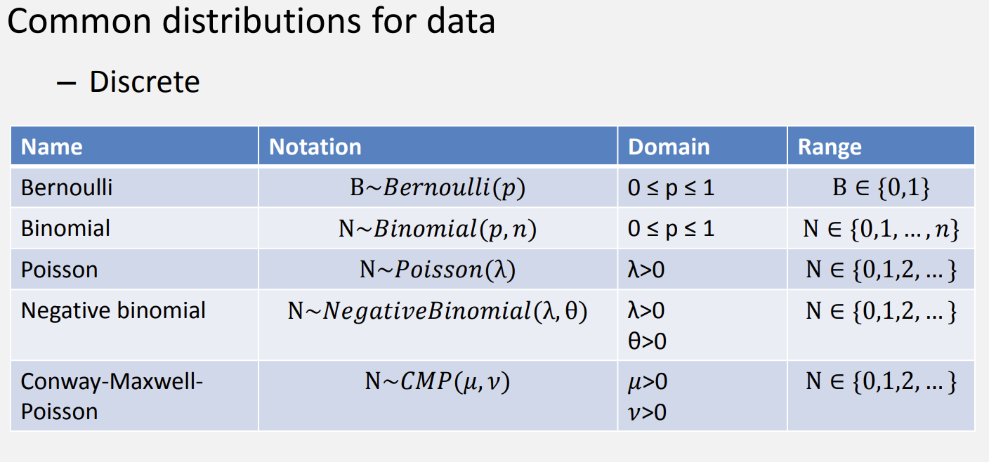
Thinking about distributions
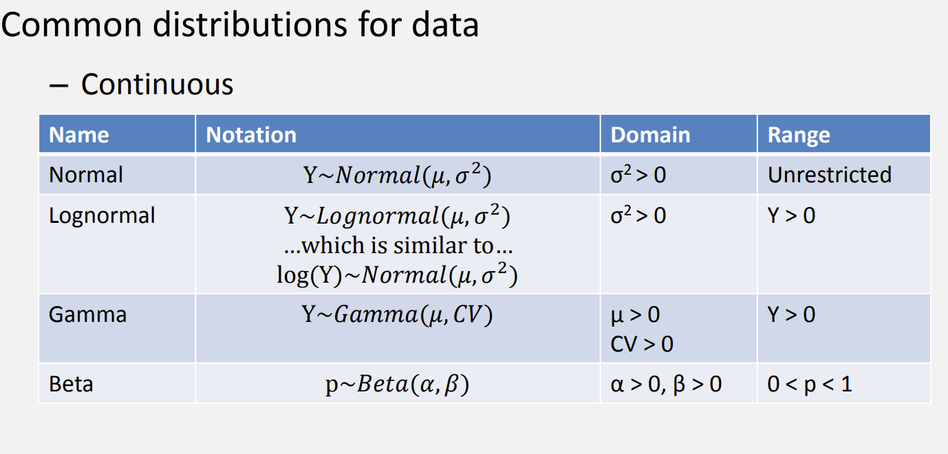
Justin Bois’ Distribution explorer
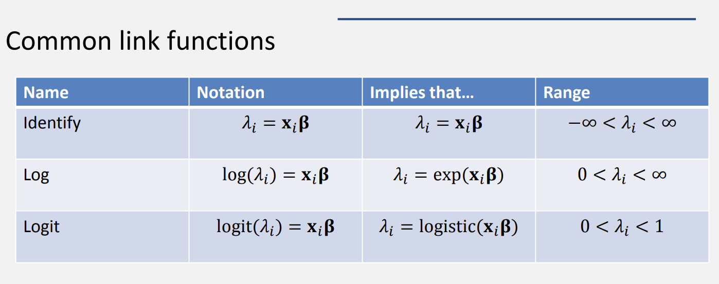
Thinking about link functions
Why you should care part I
- GLM concept gives you considerable creative freedom in combining the three components
- However, there are typically pairs of response distributions and link functions that go well together
- These are called canonical link functions
- Identity link for normal responses
- Log link for Poisson responses
- Logit link for binomial or Bernoulli responses
- However, there are typically pairs of response distributions and link functions that go well together
see Chapter 3, Kery and Royle 2016
Why you should care part II
- Bernoulli/binomial: survival, maturity, presence/absence, data either 0 or 1
- Poisson: abundance, recruitment, unbounded counts [0, Inf]
- Many exciting ecological models can be viewed as coupled GLMs
- GLMs are defined for all members of statistical distributions belonging to the so-called “exponential family” (McCullagh and Nelder 1989; Dobson and Barnett 2008)
- normal, Poisson, binomial/Bernoulli, multinomial, beta, gamma, lognormal, exponential, and Dirichlet
- Principles of linear modeling can be carried over to models other than normal linear regression 😎
see Chapter 3, Kery and Royle 2016
The Poisson GLM for unbounded counts
\[ \begin{array}{c} C_{i} \sim \operatorname{Poisson}\left(\lambda_{i}\right) \\ \log \left(\lambda_{i}\right)=X_{i,j} \cdot \mathbf{\beta_{j}} \end{array} \]
\(C\) is count of observation \(i\), \(X_{i,j}\) is a design matrix, \(j\) is number of columns, \(\mathbf{\beta}_{j}\) is a vector of parameters
simulate Poisson data in R:
  [1] 12 20 19 16  9 16 17 17 13 20 16 12 13 13 15 11 18 17 18 18 15  7 16 19 12
 [26] 13 16 20 14 16 14  9 18 13 19 13 21 17 13 11 12  8 17 14 18 16 12 11 20 22
 [51] 13 10 10 24 14 17 15 12  9 20 15 23 16 12 14 17 19 15 14 11 12 19 17 14 13
 [76] 13 18 13 19 17 20 11 19 17 21 17 10 15 18 18 11 11 10 21 17 18 16 21 12 15
The Poisson GLM for unbounded counts
\[ \begin{array}{c} C_{i} \sim \operatorname{Poisson}\left(\lambda_{i}\right) \\ \log \left(\lambda_{i}\right)=X_{i,j} \cdot \mathbf{\beta_{j}} \end{array} \]
\(C\) is count of observation \(i\), \(X_{i,j}\) is a design matrix, \(j\) is number of columns, \(\mathbf{\beta}_{j}\) is a vector of parameters
log-probability mass of Poisson count data in R:
The Poisson GLM for unbounded counts
\[ \begin{array}{c} C_{i} \sim \operatorname{Poisson}\left(\lambda_{i}\right) \\ \log \left(\lambda_{i}\right)=X_{i,j} \cdot \mathbf{\beta_{j}} \end{array} \]
- Assumptions
- The mean and variance of the Poisson distribution are equal
- Almost never holds and usually requires a negative binomial or another model structure
- Causes of over/under dispersion are complex
see Chapter 3, Kery and Royle 2016; Zuur et al. 2017
Testing for over- or under-dispersion: Poisson GLM
- mean = variance = \(\lambda\)
- Another way: Bayesian p-value
- Idea: define a test statistic and compare the posterior distribution of that statistic for the original data to the posterior distribution of that test statistic for “replicate” datasets
- Note we could also use graphical posterior predictive checks
Gelman et al. 2006; see Chapter 3, Kery and Royle 2016; Zuur et al. 2017
Bayesian p-value
- Pearson residuals:
\[ D\left(y_{i}, \theta\right)=\frac{\left(y_{i}-\mathrm{E}\left(y_{i}\right)\right)}{\sqrt{\operatorname{Var}\left(y_{i}\right)}} . \]
- Begin by calculating the sum of squared residuals (our test statistic) for the observed data:
\[ T(\mathbf{y}, \theta)=\sum_{i} D\left(y_{i}, \theta\right)^{2} \]
Bayesian p-value
- Next, we calculate the same statistic for replicate (simulated) datasets
\[ T\left(\mathbf{y}^{\text {new }}, \theta\right)=\sum_{i} D\left(y_{i}^{\text {new }}, \theta\right)^{2} \]
- Bayesian p-value is simply the posterior probability \(\operatorname{Pr}\left(T\left(\mathbf{y}^{\text {new }}\right)>T(\mathbf{y})\right)\)
- Should be close to 0.5 for a good model, too near 0 or 1 indicates lack of fit (somewhat subjective)
see Chapter 3, Kery and Royle 2016; Zuur et al. 2017
The binomial GLM for bounded counts or proportions
- Often have counts bounded by an upper limit
- Number of successful breeding pairs cannot be higher than all observed breeding pairs
- Proportion of nestlings surviving
- These types of data require the binomial GLM
Kery and Schaub 2012
The binomial GLM for bounded counts or proportions
- Random part of the response (statistical distribution)
\[ C_{i} \sim \operatorname{Binomial}\left(N_{i}, p_{i}\right) \]
- Link of the random and systematic bit (logit link):
\[ \operatorname{logit}\left(p_{i}\right)=\log \left(\frac{p_{i}}{1-p_{i}}\right)=\eta_{i} \]
- Systematic part (linear predictor):
\[ \eta_{i}=\beta_{0}+\beta_{1}{ }^{*} X_{i}+\beta_{2}{ }^{*} X_{i}^{2} \]
The binomial GLM for bounded counts or proportions
\[ C_{i} \sim \operatorname{Binomial}\left(N_{i}, p_{i}\right) \]
\[ \operatorname{logit}\left(p_{i}\right)=\log \left(\frac{p_{i}}{1-p_{i}}\right)=\eta_{i} \]
\[ \eta_{i}=\beta_{0}+\beta_{1}{ }^{*} X_{i}+\beta_{2}{ }^{*} X_{i}^{2} \]
where \(p_{i}\) is expected proportion on arithmetic scale and is mean response of each of the observed \(N_{i}\) trials
\(\eta_{i}\) is the same proportion but on the logit-link scale
The binomial GLM for bounded counts or proportions
\[ \operatorname{logit}\left(p_{i}\right)=\log \left(\frac{p_{i}}{1-p_{i}}\right)=\eta_{i} \]
- Logit maps the probability scale (i.e., range 0 to 1) to the entire real line (i.e., -\(\infty\) to \(\infty\))
- The rest of the model (linear predictor) is up to you, your data, your questions, and your imagination
Kery and Schaub 2012
Overdispersion and underdispersion in the binomial distribution
- Note that the binomial distribution variance is equal to
\[ N \cdot p \cdot (1-p) \]
- Need to check the binomial for under and over dispersion similar to how we check for the Poisson
- See this paper for some useful logistic regression checks
In-class exercise
In-class exercise
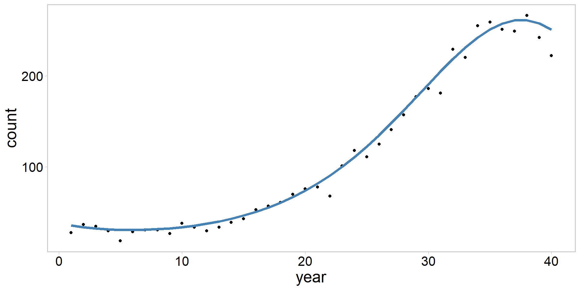
- Let’s simulate a Poisson GLM, where we model peninsular homing clam 🥟 counts as a function of year:
\[ \begin{array}{c} C_{i} \sim \operatorname{Poisson}\left(\lambda_{i}\right) \\ \log \left(\lambda_{i}\right)=\beta_{0}+\beta_{1} \cdot \operatorname{year}_{i} +\beta_{2} \cdot \operatorname{year}_{i}^2 + \beta_{3} \cdot \operatorname{year}_{i}^3 \end{array} \]
- Clam counts follow a cubic polynomial function of time
- Note this equation is still linear in the predictors
- Where do we begin?
Kery and Schaub 2012
Peninsular homing clams 🥟: simulating fake data
- Let’s get it started (in here)
- Exercise: see if you can generate fake data for this model
- Start by calculating the systematic component, then apply the link function, and lastly generate random deviates according to the Poisson distribution
Homing clam simulation solution 🥟
Coding the 🥟 model in Stan
- Assume Normal(0, 10) priors for everything
- Should look similar to the simulation code
- Hint: you will get a funny error message and we will work through it as a group
Writing the clams.stan file 🥟
- Work together to get this model estimating
Go to solution files
Summary and Recap
- We have covered much ground
- Statistical models as response = deterministic + random
- ANCOVA
- Introduced GLMs, which allow us to model data coming from distributions other than the normal
- Examined Poisson and Binomial GLMs
- Talked about dispersion
- This material lays the foundation for more complicated models
References
- Gelman et al. 2015. Stan: A probabilistic programming language for Bayesian inference and optimization
- Gelman et al. 2006. Bayesian Data Analysis.
- Gelman and Hill 2007. Data analysis using regression and multilevel models
- Hilbe et al. 2017. Bayesian models for Astrophysical data
- Kery 2010. Introduction to WinBUGS for ecologists
- Kery and Royle 2016. Applied hierarchical modeling in ecology
- Kery and Schaub. 2012. Bayesian Population Analysis using WinBUGS. Chapter 3
- McCullagh and Nelder 1989. Binary data. In Generalized linear models (pp. 98-148). London: Chapman and Hall. 511 pp
- Zuur et al. 2017. Beginner’s Guide to spatial, temporal, and spatial-temporal ecological data analysis with R-INLA. Highland Statistics Ltd.