Runtime warnings, errors, and debugging in R and Stan
FW 891
Click here to view presentation online
13 September 2023
Purpose
- Talk through some common errors and warning messages in Stan
- Most of this is available on the Stan webpage
- Can be useful for debugging or improving models
- How I debug Stan files (probably the only way)
- How I debug R code (not the only way)
Runtime warnings and convergence problems webpage and cmdstan documentation:
https://mc-stan.org/misc/warnings.html
Overview
- Stan throws a range of diagnostics, and throws warnings or errors for anything suspicious
- Some of these are more important than others, but in general having an understanding of these warnings and errors can help you debug models or figure out problems with your model
- Figuring out what’s going on is as much an art as science
The folk theorem of statistical computing
- This is a pithy rule that originated from Andrew Gelman (author of Bayesian Data Analysis). It is paraphrased as
“When you have computational problems, often there is a problem with your model [rather than the software]”—— Andrew Gelman
Types of warnings
- Divergent transitions after warmup
- Exceptions thrown when Hamiltonian proposal rejected
- R-hat
- Bulk and Tail ESS
- Maximum treedepth
- BFMI low
Divergent transitions after warmup
- Probably the most important warning
- Commonplace with mixed effects models
- Hamiltonian Monte Carlo provides internal checks on efficiency and accuracy
- These come free, arising from constraints of the physics simulation
- Recall that HMC simulates a frictionless particle
- In any given transition, total energy at the start of a simulation should be equal to the total energy at the end
- When this doesn’t happen, the energy is “divergent”
- often means the posterior distribution is very steep in some region of parameter space, hard to sample
McElreath 2023
Divergent transitions after warmup
- Critical to recognize that divergent transitions cannot be safely ignored if completely reliable inference is desired
- Proceed at your own risk: you may not be faithfully representing the posterior uncertainty if you ignore DTs
- If you only get a few divergences and good Rhat values and ESS, the resulting posterior is often good enough to move forward
- There are cases where a small number of divergences without any pattern in their locations can be shown to be unimportant, but this requires a lot of simulation and math
- The bottom line is your inferences may be biased if there are DTs after warmup
Divergent transitions after warmup
How to deal with DTs:
- Double check the code (even coding errors can cause DTs)
- Increase the adaptation target acceptance statistic,
adapt_delta, > 0.8- Must be between 0,1, so values >> 0.999 have diminishing returns
- The step size used by the numerical integrator underlying Stan is a function of
adapt_delta, so this results in a smaller step size and (sometimes) fewer divergences
- If (2) does not work, consider priors or reparameterizing the model
- Plot the data, hone in on where in the model the divergent transitions are occurring
- Lots of pairs plots, divergent transition plots
- DTs can indicate many things, and often reveal information about your experimental design or the lack of information content contained in your data
- Weep 😭
Exceptions thrown when Hamiltonian proposal rejected
First warning indicates that the standard deviation parameter of the normal distribution is zero, but it must be positive for Stan to compute the density function
The second message indicates that the gradient of the target (as computed by Stan’s automatic differention) is infinite, indicating numerical problems somewhere in the model but unfortunately without clear information about where exactly.
Exceptions thrown when Hamiltonian proposal rejected
- Note: it is possible that even in a correctly specified model a numerical inaccuracy is occasionally seen, especially during warmup
- For example, scale parameter with zero lower bound can still become numerically indistinguishable from zero
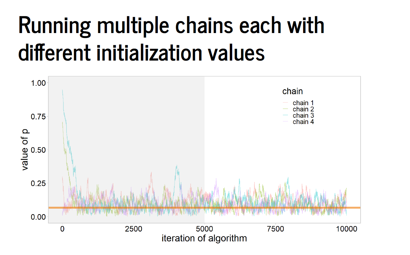
Split-\(\widehat{R}\) aka Rhat
- This statistic compares means and variances of the chains
- Remember, we use several chains to make convergence diagnostics easier, starting chains at different starting points
- Values < 1.1 often sufficient
- We remove draws from the beginning of the chains and run the chains long enough so that it is not possible to distinguish where each chain started
- A fair amount of math behind this (see link below)
- We remove draws from the beginning of the chains and run the chains long enough so that it is not possible to distinguish where each chain started
Some slides from Aki Vehtari on convergence to a common posterior
See here:
Nonconvergence
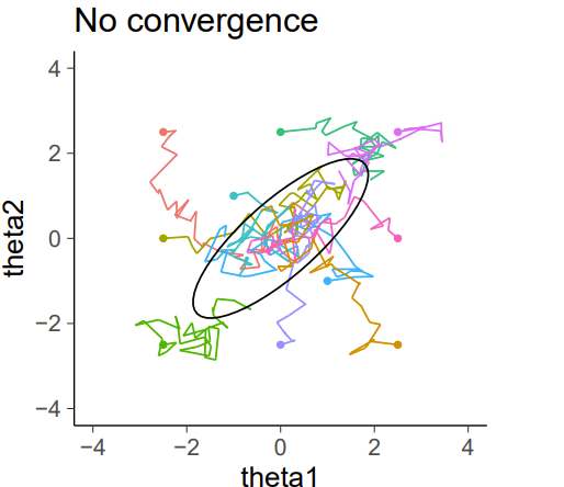
Nonconvergence viewed another way

Visually converged chains

High \(\widehat{R}\) values
- Indicate the chains have not mixed well
- Good reasons to NOT think of them as being fully representative of the posterior = bad inference
- When there are also DTs in the model, just another symptom of problematic geometry that caused the divergences
- If high \(\widehat{R}\) without other warnings, often associated with posteriors that have multiple, well-separated modes
- Running chains longer may help
https://mc-stan.org/misc/warnings.html; Gelman et al. 2003
Bulk and tail Effective Sample Size (ESS)
- Roughly speaking, ESS tells you how many independent draws contain the same amount of information as the dependent sample obtained by the MCMC algorithm
- Higher is better
- For final analyses, Stan recommends bulk-ESS > 100x the number of chains
- 4 chains, want rank-normalized ESS of at least 400
- Early in an analysis, ESS > 20 is fine
Bulk and tail Effective Sample Size (ESS)
- Tail-ESS computes the minimum of the ESS of the 5th and 95th quantiles
- Warnings about tail-ESS can help diagnose slow mixing in the tails
- These warnings are often accompanied by large \(\widehat{R}\) values
- Useful quick summary, but for final results it can be useful to check Monte Carlo standard error for quantities of interest (not shown)
- Introduce thinning, and the only reason to do it
https://mc-stan.org/docs/reference-manual/effective-sample-size.html
Maximum treedepth warnings
- Not as serious as other warnings
- DTs, high \(\widehat{R}\) and low ESS are a validity concern
- Maximum treedepth warnings are an efficiency concern
- Configuring the NUTS sampler (variant of HMC used by Stan) involves putting a cap on the number of simulation steps it evaluates during each iteration
- This is controlled by the
max_treedepthparameter, where maximum number of steps = 2^max_treedepth
- This is controlled by the
- If you are only getting this warning and other diagnostics are good, likely safe to ignore (but you may lose out on efficiency)
<https://mc-stan.org/misc/warnings.html#bulk-and-tail-ess >
Bayesian Fraction of Missing Information (BFMI)
Example:
- There is an
energy__output from Stan’s samplers is used to diagnose the accuracy of HMC - Implication of this warning is that HMC is not exploring the posterior well, in particular the tails of the posterior
- Run the model longer or reparameterize your model
- Mathematically dense (see Betancourt 2016) https://arxiv.org/pdf/1604.00695.pdf
Debugging Stan code
- Stan provides
print()statements that can print literal strings and the values of expressions print(): accepts any number of arguments
- Each time the loop body is executed, it will print the string “loop iteration:” (with the trailing space), followed by the value of the expression n, followed by a new line
https://mc-stan.org/docs/reference-manual/print-statements.html
Useful things to do with print()
- Very useful for debugging, particularly when coupled with
target()target()is the log density accumulator, and is actually a reserved word in Stan
https://mc-stan.org/docs/reference-manual/print-statements.html
Debugging R code
- Ten minute warp-speed lesson on debugging in R
- Several ways to do this, but here we’ll do a demo of the functions
traceback()andbrowser()
traceback()
- identifies which function generated the error
browser()
- Abstract and not well implemented (Belinsky, pers comm 2023)
- This is what I (Cahill) mainly use to debug R code
- Interrupts the execution of an expression and allow the inspection of the environment where browser was called from
browser()
- Put a
browser()in it to win it
https://stat.ethz.ch/R-manual/R-devel/library/base/html/browser.html
browser()
- Go to R to demonstrate how to use
- Note this works with for-loops and other horrid things
Summary and outlook
- Went through some common Stan runtime warnings and error messages
- Discussed that some checks are about the validity of inferences while others are about efficiency
- Debugging Stan code via
print()statements - Debugging R code via
traceback()andbrowser() - Next few weeks, move into nonlinear and mixed effects modeling (where we will experience some of these warnings/issues)
References
Betancourt, M. 2016. Diagnosing suboptimal cotangent disintegrations in Hamiltonian Monte Carlo. https://arxiv.org/pdf/1604.00695.pdf
Gelman et al. 2003. Bayesian Data Analysis.
McElreath 2023. Statistical Rethinking. Second Edition.
Stan documentation. 2023. https://mc-stan.org/docs/reference-manual/index.html