Fitting nonlinear ecological models in Stan
FW 891
Click here to view presentation online
18 September 2023
Nonlinear modeling is like wandering down a sketchy alley with no end in sight

Where do nonlinear model equations come from?

Visualizing that model in R
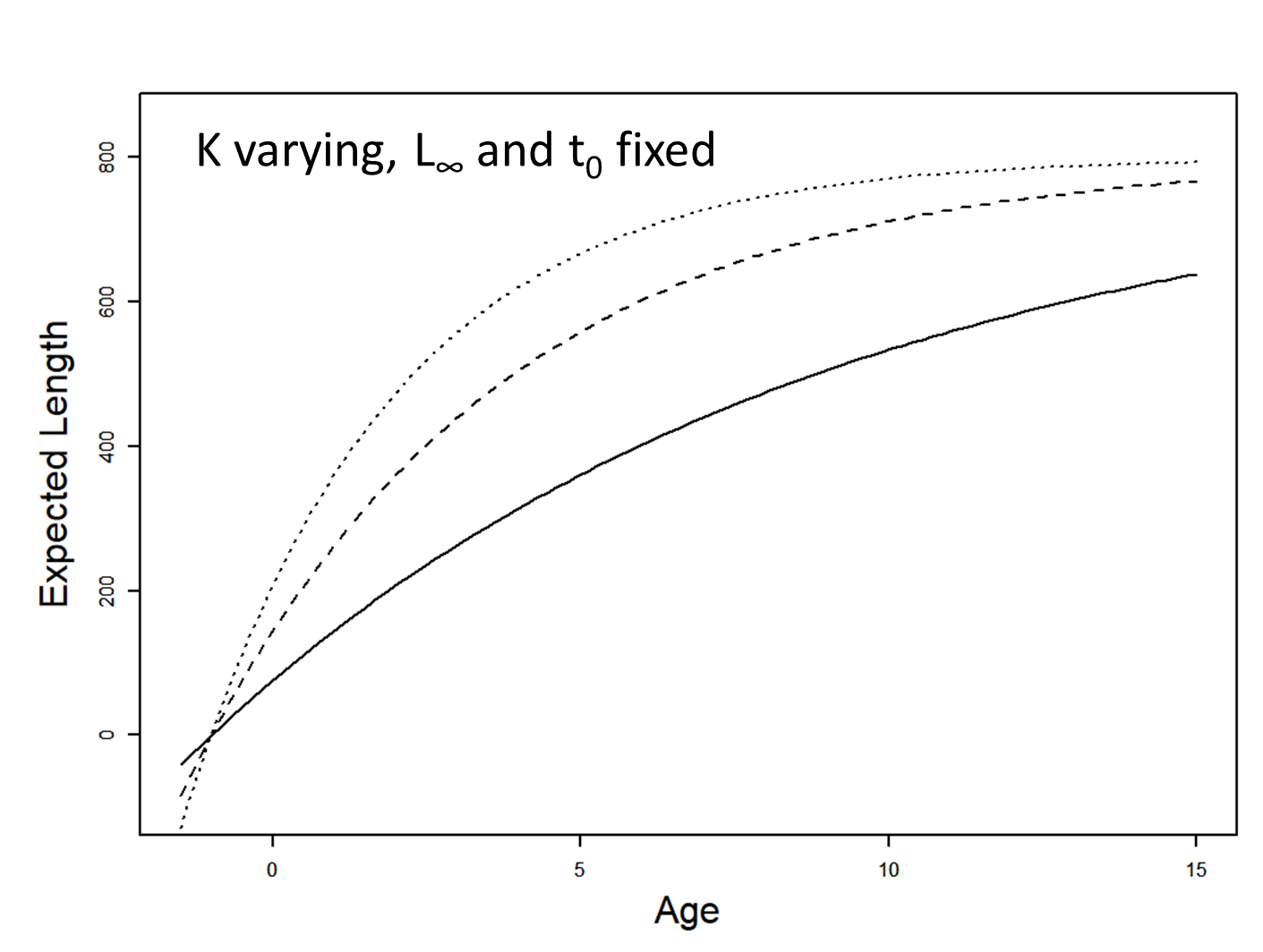
Visualizing the model
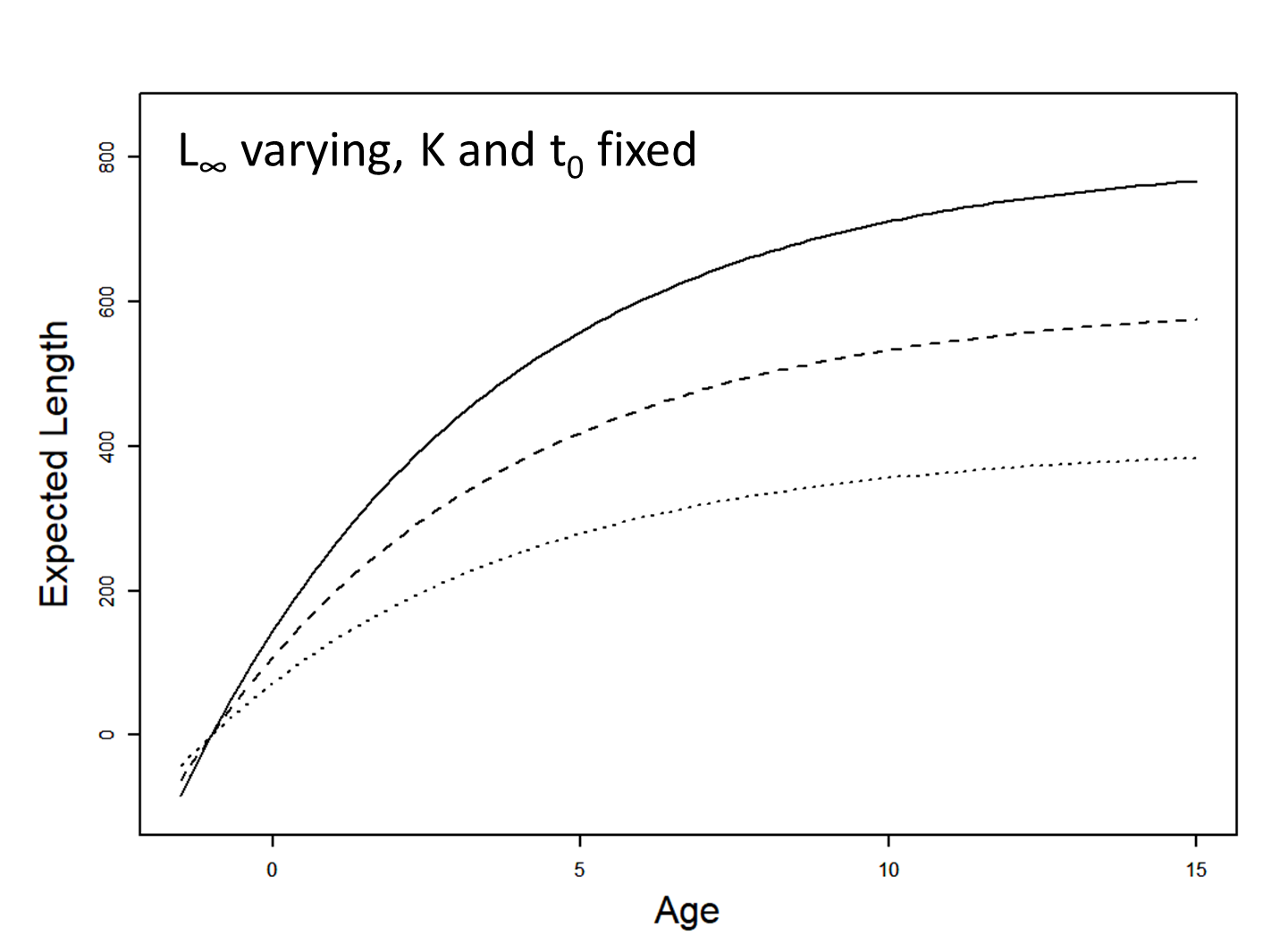
Visualizing the model
Some challenges associated with nonlinear modeling
- Requires a better handle on both math/calculus and numerical computing
- Need to understand the properties of a variety of probability distributions and deterministic response functions (Link and Barber 2010; Bolker et al. 2013)
- Even after a model has been properly formulated, it can be difficult to fit to data and estimate parameters
- No gaurantees of global optimum, which means model checking and priors even more important
- There is no “dummies” guide to nonlinear ecological model fitting
- Critical to have good starting values, priors, tests with simulated data, etc.


Advice (from Bolker et al. 2013)
- Most complex models are extensions of simpler models
- Thus, often makes sense to fit reduced versions of the model and build up working code blocks
- Can use reduced models to get good starting values for more complex models in some cases
- Choose a subset of your data that makes your code run fast during the debugging stage
- Keep It Simple Stupid (KISS), at least to start

Specific suggestions to overcome problems
- Initially omit complexities of the model as much as possible (random effects, zero inflation, imprefect detection)
- Hold some parameters constant or set strong priors to restrict parameters to a narrow range
- Reduce the model to a simpler form by setting some parameters, especially exponents or shape parameters, to null values
- e.g., try a Poisson model before a negative binomial model
- or an exponential suvival model before a Gamma model

In class examples
von Bertalanffy model to estimate fish growth (fake data where I know truth but you do not; easy)
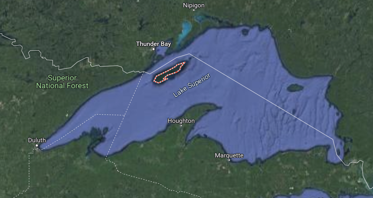
Type-II predator-prey model for wolves and moose (real data from Isle Royale; intermediate)
Schaefer surplus-production model to estimate maximum sustainable yield (real data from south Atlantic Albacore Tuna; hard)


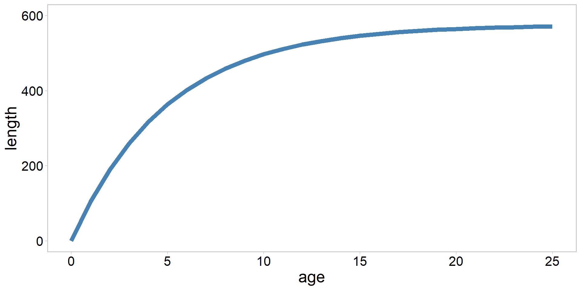
The von Bertalanffy growth model

The von Bertalanffy growth model
Will a 21 inch minimum length limit work?
The model: \[ \begin{array}{l} L_{i}=L_{\infty}\left(1-e^{-K\left(a_{i}-t_{0}\right)}\right)+\varepsilon_{i} \\ \varepsilon_{i} \stackrel{i i d}{\sim} N\left(0, \sigma^{2}\right) \end{array} \]
Fit this model using Stan
Evaluate your model
Predator-prey models
The Isle Royale natural experiment
Tuna sustainability in the south Atlantic
Recap
- We have introduced nonlinear models
- Hopefully it has been conveyed that these things are tricksy, but really critical for many important ecological and resource mgmt problems
- Up next…