Introduction to hierarchical (mixed-effects) models part II

FW 891
Click here to view presentation online

Christopher Cahill

27 September 2023

Purpose

• Another look at how we specify a joint posterior for hierarchical models (maths)
  • Demonstrate the importance of conditional independence
• Demonstrate a hierarchical binomial survival model for quail stocking survival

A hierarchical model

\[ \begin{aligned} y_{i} & \stackrel{i n d}{\sim} p\left(y \mid \theta_{i}\right) \\ \theta_{i} & \stackrel{i i d}{\sim} p(\theta \mid \phi) \\ \phi & \sim p(\phi) \end{aligned} \]

A hierarchical model

\[ \begin{aligned} y_{i} & \stackrel{i n d}{\sim} p\left(y \mid \theta_{i}\right) \\ \theta_{i} & \stackrel{i i d}{\sim} p(\theta \mid \phi) \\ \phi & \sim p(\phi) \end{aligned} \]

• \(y_{i}\) is observed data

A hierarchical model

\[ \begin{aligned} y_{i} & \stackrel{i n d}{\sim} p\left(y \mid \theta_{i}\right) \\ \theta_{i} & \stackrel{i i d}{\sim} p(\theta \mid \phi) \\ \phi & \sim p(\phi) \end{aligned} \]

• \(y_{i}\) is observed data
• \(\theta=\left(\theta_{1}, \ldots, \theta_{n}\right) \text { and } \phi\) are parameters

A hierarchical model

\[ \begin{aligned} y_{i} & \stackrel{i n d}{\sim} p\left(y \mid \theta_{i}\right) \\ \theta_{i} & \stackrel{i i d}{\sim} p(\theta \mid \phi) \\ \phi & \sim p(\phi) \end{aligned} \]

• \(y_{i}\) is observed data
• \(\theta=\left(\theta_{1}, \ldots, \theta_{n}\right) \text { and } \phi\) are parameters
• Only \(\phi\) has a prior that is set (assumed)

Mathematical support puppies

Posterior distribution for hierarchical models

• The joint posterior distribution of interest in hierarchical models is

\[ p(\theta, \phi \mid y) \]

Posterior distribution for hierarchical models

• The joint posterior distribution of interest in hierarchical models is

\[ p(\theta, \phi \mid y) \]

• Apply Bayes rule

Posterior distribution for hierarchical models

• The joint posterior distribution of interest in hierarchical models is

\[ p(\theta, \phi \mid y) \propto p(y \mid \theta, \phi) p(\theta, \phi) \]

• Apply Bayes rule

Posterior distribution for hierarchical models

• The joint posterior distribution of interest in hierarchical models is

\[ p(\theta, \phi \mid y) \propto p(y \mid \theta, \phi) p(\theta, \phi)=p(y \mid \theta) p(\theta \mid \phi) p(\phi) \]

• Apply Bayes rule

• We can also break this joint distribution down into a conditional distribution of \(\theta\) given \(\phi\)

Posterior distribution for hierarchical models

• The joint posterior distribution of interest in hierarchical models is

\[ p(\theta, \phi \mid y) \propto p(y \mid \theta, \phi) p(\theta, \phi)=p(y \mid \theta) p(\theta \mid \phi) p(\phi) \]

• Apply Bayes rule

• We can also break this joint distribution down into a conditional distribution of \(\theta\) given \(\phi\)

  • Do this using conditional probability rules

Posterior distribution for hierarchical models

• The joint posterior distribution of interest in hierarchical models is

\[ p(\theta, \phi \mid y) \propto p(y \mid \theta, \phi) p(\theta, \phi)=p(y \mid \theta) p(\theta \mid \phi) p(\phi) \]

Posterior distribution for hierarchical models

• The joint posterior distribution of interest in hierarchical models is

\[ p(\theta, \phi \mid y) \propto p(y \mid \theta, \phi) p(\theta, \phi)=p(y \mid \theta) p(\theta \mid \phi) p(\phi) \]

• We may also care about the marginal posterior of \(\theta\):

Posterior distribution for hierarchical models

• The joint posterior distribution of interest in hierarchical models is

\[ p(\theta, \phi \mid y) \propto p(y \mid \theta, \phi) p(\theta, \phi)=p(y \mid \theta) p(\theta \mid \phi) p(\phi) \]

• We may also care about the marginal posterior of \(\theta\):

\[ p(\theta \mid y)=\int p(\theta, \phi \mid y) d \phi \]

Posterior distribution for hierarchical models

• The joint posterior distribution of interest in hierarchical models is

\[ p(\theta, \phi \mid y) \propto p(y \mid \theta, \phi) p(\theta, \phi)=p(y \mid \theta) p(\theta \mid \phi) p(\phi) \]

• We may also care about the marginal posterior of \(\theta\):

\[ p(\theta \mid y)=\int p(\theta, \phi \mid y) d \phi \]

• Or instead the marginal distribution of \(\phi\):

\[ p(\phi \mid y)=\int p(\theta, \phi \mid y) d \theta \]

Posterior distribution for hierarchical models

• The joint posterior distribution of interest in hierarchical models is

\[ p(\theta, \phi \mid y) \propto p(y \mid \theta, \phi) p(\theta, \phi)=p(y \mid \theta) p(\theta \mid \phi) p(\phi) \]

• We may also care about the marginal posterior of \(\theta\):

\[ p(\theta \mid y)=\int p(\theta, \phi \mid y) d \phi \]

• Or instead the marginal distribution of \(\phi\):

\[ p(\phi \mid y)=\int p(\theta, \phi \mid y) d \theta \]

• \(p(unknowns|knowns) \propto \text { assumptions you make }\)

Survival of stocked quail chicks

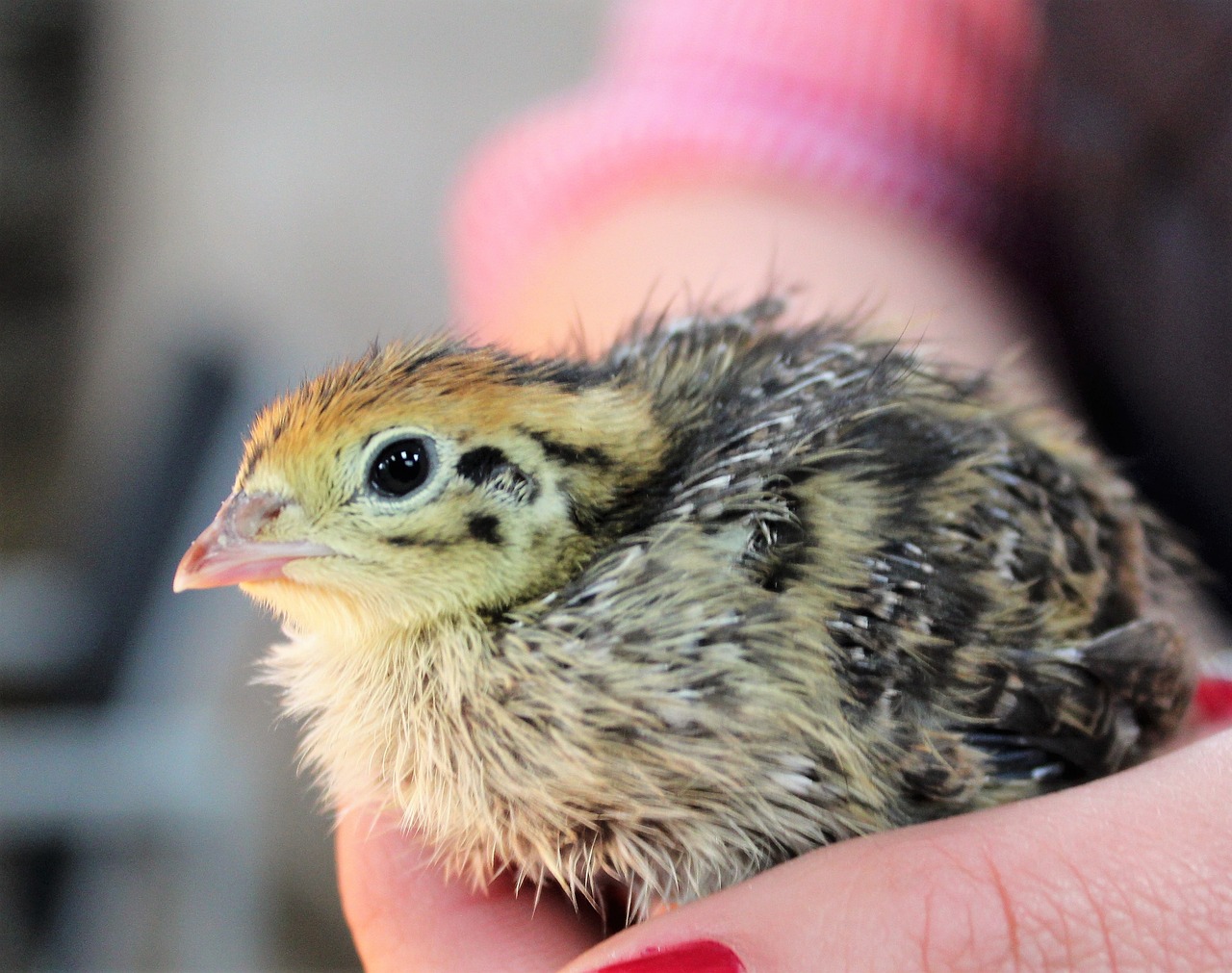
Survival of stocked quail chicks 🐥

• Juvenile quail have relatively high mortality rates
• Managers want to conduct an management experiment where chicks are released into 100x100m penned-enclosures to determine chick survival in their region
  • Released between 6 and 20 chicks in on 11 farms
  • Go back one month later and see how many survive

The hierarchical fluff chicken survival model 🐥

\[ \begin{array}{ll} Y_{i} & \stackrel{i n d}{\sim} \operatorname{Bin}\left(n_{i}, \theta_{i}\right) \\ \theta_{i} & \stackrel{i i d}{\sim} \operatorname{Be}(\alpha, \beta) \\ \alpha, \beta & \sim p(\alpha, \beta) \end{array} \]

• \(Y_{i}\) is number of chicks alive at end of month
• \(n_{i}\) is number of chicks released at start of month
• \(\theta_{i}\) is chick survival at farm i
• \(\alpha\) and \(\beta\) are the parameters of the Beta distribution

The hierarchical fluff chicken survival model 🐥

\[ \begin{array}{ll} Y_{i} & \stackrel{i n d}{\sim} \operatorname{Bin}\left(n_{i}, \theta_{i}\right) \\ \theta_{i} & \stackrel{i i d}{\sim} \operatorname{Be}(\alpha, \beta) \\ \alpha, \beta & \sim p(\alpha, \beta) \end{array} \]

Also note that \(\phi\) from previous slides is now \(\phi = (\alpha, \beta)\)

Priors for \(\alpha\) and \(\beta\)

• The interpretation of these parameters
  • \(\alpha\) is successes
  • \(\beta\) is failures
    
• A more useful parameterization in our case is
  • Beta expectation: \(\mu=\frac{\alpha}{\alpha+\beta}\)
  • Beta sample size: \(\eta=\alpha+\beta\)
• Easier to put priors on \(\mu\), \(\eta\) than \(\alpha\), \(\beta\) so we will take advantage of this

Go to the R and Stan code

The quail data and prior information

• The quail data
  • Not a ton of data
• The R script
• The Stan model

Prior information

• Bios note that the available literature indicates survival for transplanted baby quail ranges between 0.05 and 0.45

The TODO list

1. Reparameterize the beta distribution to estimate on mean \(\theta_{\mu}\) and sample size \(\eta\).
   • Note \(\alpha\) and \(\beta\) will then be derived parameters
2. Develop a prior for mean survival that places approximately 95% of its probability mass in the range 0.05 to 0.45, and a prior that is somewhat diffuse for \(\eta\) but which has most probability mass at low values
3. Develop a hierarchical model for average chick survival and farm (i.e., group) specific survival estimates given the available data
4. Plot the marginal distribution of \(\alpha\) and \(\beta\) to help put the miserable integral symbols into perspective
5. Do a prior sensitivity test to your informative prior from (1)
6. What is the probability that survival from farm two is less than average? Similarly, what is the probability that survival from farm two is less than survival from farm 6?
7. If we went to a new farm in the region and wanted to release chicks, what would our best guess be for chick survival at this farm?

Extensions

• The basic structure of a hierarchical model is \[ y \sim p(y \mid \theta) \quad \theta \sim p(\theta \mid \phi) \quad \phi \sim p(\phi) \]

• We can extend this to more than one level

\[ y \sim p(y \mid \theta) \quad \theta \sim p(\theta \mid \phi) \quad \phi \sim p(\phi \mid \psi) \quad \psi \sim p(\psi) \]

• Remember conditional independence structure

\[ p(\theta, \phi, \psi \mid y) \propto p(y \mid \theta) p(\theta \mid \phi) p(\phi \mid \psi) p(\psi) \]

Summary and outlook

• Specifically tried to talk about hierarchical models in a different (mathier) way than what we did last time
  • Did this to highlight how conditional independence plays a key role in our ability to build these models
• Built a hierarchical survival model for ditch chickens
  • This included deriving an informative prior for \(\theta_{\mu}\)
• Began to play a bit more with output from hierarchical models to generate useful quantities for management
  • Probability of chick survival at a new farm not included in the original study
• Next time, dealing with divergent transitions and varying effects

References

• Berliner, L. M. 1996, Hierarchical Bayesian time series models”, Maximum Entropy and Bayesian Methods, 15-22.

• Gelman and Hill 2007. Data analysis using regression and multilevel models

• Royle and Dorazio 2008. Hierarchical modeling and inference in ecology.

• Kery and Schaub. 2012. Bayesian Population Analysis using WinBUGS. Chapter 3

• McElreath 2023. Statistical Rethinking. Second Edition, Chapters 2 and 9.

• Punt et al. 2011. Among-stock comparisons for improving stock assessments of data-poor stocks: the “Robin Hood” approach. ICES Journal of Marine Sci.

• Jarad Niemi lecture on a very similar model from which my example is based heavily https://www.youtube.com/watch?v=nNQdvXfW73E