Pathologies in hierarchical models

FW 891
Click here to view presentation online

Christopher Cahill

16 October 2023

Purpose

Introduce some background and theoretical concepts
The Devil’s funnel (spooky seaz’n 👻)
What to do about it
Example
Example #2 (Eight schools)

Background

Many of the most exciting problems in applied statistical ecology involve intricate, high-dimensional models, and sparse data (at least relative to model complexity)

Betancourt and Girolami 2013

Background

Many of the most exciting problems in applied statistical ecology involve intricate, high-dimensional models, and sparse data (at least relative to model complexity)
In situations where the data alone cannot identify a model, significant prior information is required to draw valid inference

Betancourt and Girolami 2013

Background

Many of the most exciting problems in applied statistical ecology involve intricate, high-dimensional models, and sparse data (at least relative to model complexity)
In situations where the data alone cannot identify a model, significant prior information is required to draw valid inference
Such prior information is not limited to an explicit prior distribution, but instead can be encoded in the model construction itself 🤯

Betancourt and Girolami 2013

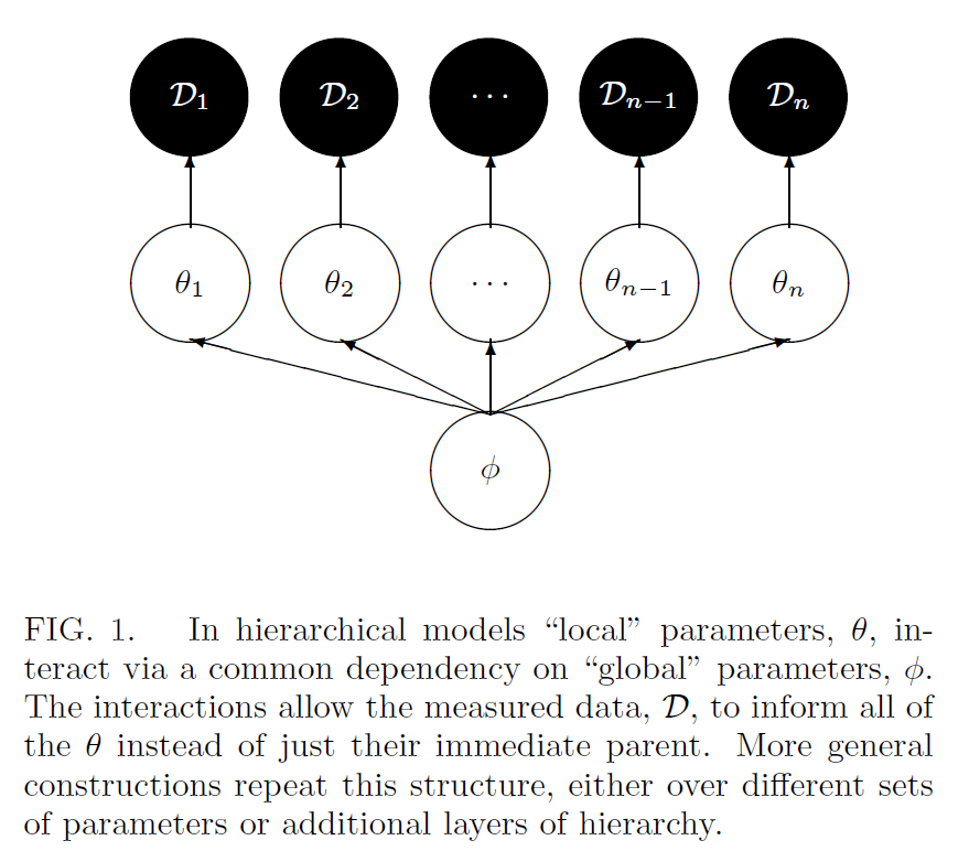
A one level hierarchical model

\[ \pi(\theta, \phi \mid \mathcal{D}) \propto \prod_{i=1}^{n} \pi\left(\mathcal{D}_{i} \mid \theta_{i}\right) \pi\left(\theta_{i} \mid \phi\right) \pi(\phi) \]

Betancourt and Girolami 2013

A one level hierarchical model

\[ \pi(\theta, \phi \mid \mathcal{D}) \propto \prod_{i=1}^{n} \pi\left(\mathcal{D}_{i} \mid \theta_{i}\right) \pi\left(\theta_{i} \mid \phi\right) \pi(\phi) \]

Hierarchical models are defined by the organization of a model’s parameters into exchangeable groups, and the resulting conditional independencies between those groups

Betancourt and Girolami 2013

A one level hierarchical model

\[ \pi(\theta, \phi \mid \mathcal{D}) \propto \prod_{i=1}^{n} \pi\left(\mathcal{D}_{i} \mid \theta_{i}\right) \pi\left(\theta_{i} \mid \phi\right) \pi(\phi) \]

Hierarchical models are defined by the organization of a model’s parameters into exchangeable groups, and the resulting conditional independencies between those groups
Can also visualize this as a directed acyclic graph (DAG)

Betancourt and Girolami 2013

Hierarchical DAG

Betancourt and Girolami 2013

A one-level hierarchical model

\[ \begin{aligned} y_{i} & \sim {N}\left(\theta_{i}, \sigma_{i}^{2}\right) \\ \theta_{i} & \sim {N}\left(\mu, \tau^{2}\right), \text { for } i=1, \ldots, I \end{aligned} \]

Betancourt and Girolami 2013

A one-level hierarchical model

\[ \begin{aligned} y_{i} & \sim {N}\left(\theta_{i}, \sigma_{i}^{2}\right) \\ \theta_{i} & \sim {N}\left(\mu, \tau^{2}\right), \text { for } i=1, \ldots, I \end{aligned} \]

In terms of the previous equations, \(\mathcal{D}=\left(y_{i}, \sigma_{i}\right), \phi=(\mu, \tau), \text { and } \theta=\left(\theta_{i}\right)\)

Betancourt and Girolami 2013

A one-level hierarchical model

\[ \begin{aligned} y_{i} & \sim {N}\left(\theta_{i}, \sigma_{i}^{2}\right) \\ \theta_{i} & \sim {N}\left(\mu, \tau^{2}\right), \text { for } i=1, \ldots, I \end{aligned} \]

In terms of the previous equations, \(\mathcal{D}=\left(y_{i}, \sigma_{i}\right), \phi=(\mu, \tau), \text { and } \theta=\left(\theta_{i}\right)\)
Call any elements of \(\phi\) global parameters

Betancourt and Girolami 2013

A one-level hierarchical model

\[ \begin{aligned} y_{i} & \sim {N}\left(\theta_{i}, \sigma_{i}^{2}\right) \\ \theta_{i} & \sim {N}\left(\mu, \tau^{2}\right), \text { for } i=1, \ldots, I \end{aligned} \]

In terms of the previous equations, \(\mathcal{D}=\left(y_{i}, \sigma_{i}\right), \phi=(\mu, \tau), \text { and } \theta=\left(\theta_{i}\right)\)
Call any elements of \(\phi\) global parameters
Call any elements of \(\theta\) local parameters

Betancourt and Girolami 2013

A one-level hierarchical model

\[ \begin{aligned} y_{i} & \sim {N}\left(\theta_{i}, \sigma_{i}^{2}\right) \\ \theta_{i} & \sim {N}\left(\mu, \tau^{2}\right), \text { for } i=1, \ldots, I \end{aligned} \]

In terms of the previous equations, \(\mathcal{D}=\left(y_{i}, \sigma_{i}\right), \phi=(\mu, \tau), \text { and } \theta=\left(\theta_{i}\right)\)
Call any elements of \(\phi\) global parameters
Call any elements of \(\theta\) local parameters
However, recognize this nomencalture breaks down in situations with more levels

Betancourt and Girolami 2013

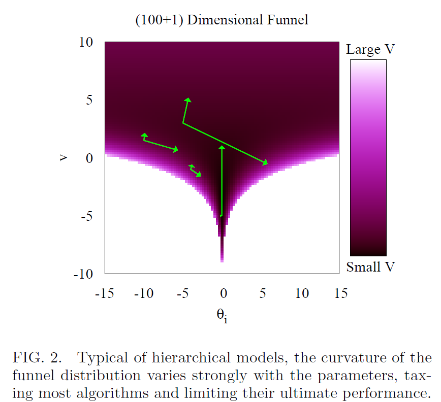
A key pathology

Unfortunately, this one-level model exhibits some of the typical pathologies of hierarchical models
Small changes in \(\phi\) induce large changes in density
When data are sparse, the density of these models looks like a “funnel”
- Region of high density but low volume, and a region of low density but high volume
However, the probability mass of these two regions is the same (or nearly so)
Any algorithm must be able to manage the dramatic variations in curvature to fully map out the posterior

Betancourt and Girolami 2013

Naive model implementations

Assuming a normal model with no data, a latent mean \(\mu\) set at zero, and a lognormal prior on the variance \(\tau^{2}=e^{v^{2}}\)

Betancourt and Girolami 2013

Naive model implementations

Assuming a normal model with no data, a latent mean \(\mu\) set at zero, and a lognormal prior on the variance \(\tau^{2}=e^{v^{2}}\)

\[ \pi\left(\theta_{1}, \ldots, \theta_{n}, v\right) \propto \prod_{i=1}^{n} N\left(x_{i} \mid 0,\left(e^{-v / 2}\right)^{2}\right) N\left(v \mid 0,3^{2}\right) \]

Betancourt and Girolami 2013

Naive model implementations

Assuming a normal model with no data, a latent mean \(\mu\) set at zero, and a lognormal prior on the variance \(\tau^{2}=e^{v^{2}}\)

\[ \pi\left(\theta_{1}, \ldots, \theta_{n}, v\right) \propto \prod_{i=1}^{n} N\left(x_{i} \mid 0,\left(e^{-v / 2}\right)^{2}\right) N\left(v \mid 0,3^{2}\right) \]

This hierarchical structure induces large correlations between \(v\) and each \(\theta_{i}\)

Betancourt and Girolami 2013

Visualizing the pathology 😈

Some things worth noting

There is position dependence in the correlation structure, i.e., correlation changes depending on where you are located in the posterior

Betancourt and Girolami 2013

Some things worth noting

There is position dependence in the correlation structure, i.e., correlation changes depending on where you are located in the posterior
No global correction, like rotating or rescaling will solve this problem!

Betancourt and Girolami 2013

Some things worth noting

There is position dependence in the correlation structure, i.e., correlation changes depending on where you are located in the posterior
No global correction, like rotating or rescaling will solve this problem!
Often manifests as a divergent transition in Stan, as HMC cannot accurately explore the posterior

Betancourt and Girolami 2013

How can we fix this problem?

Remember that the prior information we include in an analysis is not only limited to the choice of an explict prior distribution

Betancourt and Girolami 2013

How can we fix this problem?

Remember that the prior information we include in an analysis is not only limited to the choice of an explict prior distribution
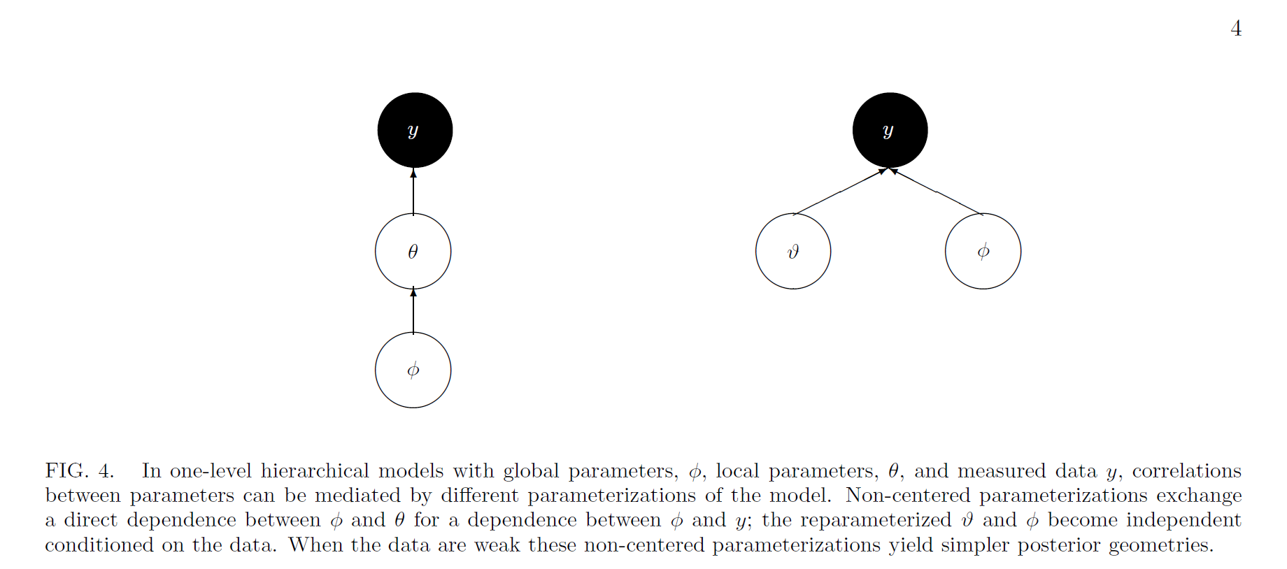
The dependence between layers in our model can actually be broken up by reparameterizing the existing parameters into a so-called “non-centered” parameterization
- Think about the DAG Betancourt and Girolami 2013

How can we fix this problem?

Remember that the prior information we include in an analysis is not only limited to the choice of an explict prior distribution
The dependence between layers in our model can actually be broken up by reparameterizing the existing parameters into a so-called “non-centered” parameterization
- Think about the DAG
Non-centered parameterizations factor certain dependencies into deterministic transformations between the layers, leaving the actively sampled variables uncorrelated

Betancourt and Girolami 2013

Centered vs. non-centered model maths

Centered model: \[ \begin{aligned} y_{i} & \sim {N}\left(\theta_{i}, \sigma_{i}^{2}\right) \\ \theta_{i} & \sim {N}\left(\mu, \tau^{2}\right), \end{aligned} \]

Non-centered analog:

Betancourt and Girolami 2013

Centered vs. non-centered model maths

Centered model: \[ \begin{aligned} y_{i} & \sim {N}\left(\theta_{i}, \sigma_{i}^{2}\right) \\ \theta_{i} & \sim {N}\left(\mu, \tau^{2}\right), \end{aligned} \]

Non-centered analog:

\[ \begin{aligned} y_{i} & \sim N\left(\vartheta_{i} \tau+\mu, \sigma_{i}^{2}\right) \\ \vartheta_{i} & \sim N(0,1). \end{aligned} \]

Betancourt and Girolami 2013

Centered vs. non-centered model maths

Centered model: \[ \begin{aligned} y_{i} & \sim {N}\left(\theta_{i}, \sigma_{i}^{2}\right) \\ \theta_{i} & \sim {N}\left(\mu, \tau^{2}\right), \end{aligned} \]

Non-centered analog:

\[ \begin{aligned} y_{i} & \sim N\left(\vartheta_{i} \tau+\mu, \sigma_{i}^{2}\right) \\ \vartheta_{i} & \sim N(0,1). \end{aligned} \]

Key point: NCP shifts correlation from the latent parameters to data

Betancourt and Girolami 2013

Centered vs. non-centered model DAG

Betancourt and Girolami 2013

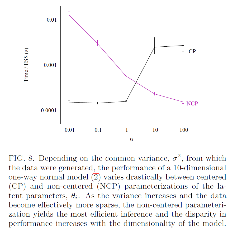
When does NCP help?

Betancourt and Girolami 2013

Example

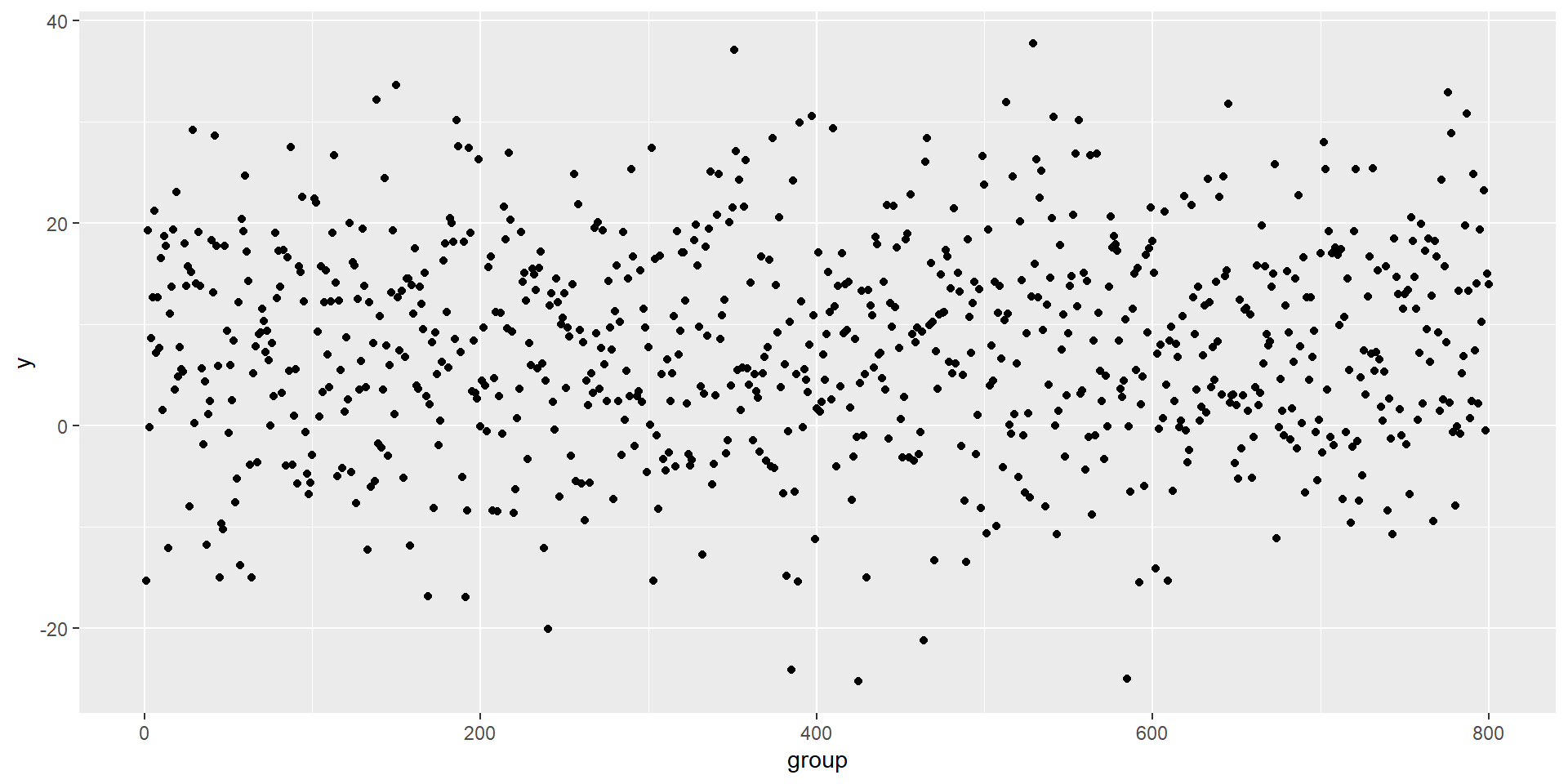
Example

consider the one-way normal model with 800 latent \(\theta_{i}\)
constant measurement error \(\sigma_{i} = \sigma = 10\)
latent parameters are \(\mu = 8, \tau = 3\)
\(\theta_{i}\) and \(y_{i}\) sampled randomly

Betancourt and Girolami 2013

Example

consider the one-way normal model with 800 latent \(\theta_{i}\)
constant measurement error \(\sigma_{i} = \sigma = 10\)
latent parameters are \(\mu = 8, \tau = 3\)
\(\theta_{i}\) and \(y_{i}\) sampled randomly

Add weakly informative priors to this generative likelihood

\[ \begin{array}{l} \pi(\mu)=N\left(0,5^{2}\right) \\ \pi(\tau)=\text { Half-Cauchy }(0,2.5) . \end{array} \]

Betancourt and Girolami 2013

Example, centered vs. noncentered

The centered parameterization of this model can be written as

\[ \begin{aligned} y_{i} & \sim N\left(\theta_{i}, \sigma_{i}^{2}\right) \\ \theta_{i} & \sim N\left(\mu, \tau^{2}\right), \text { for } i=1, \ldots, 800 \end{aligned} \]

Betancourt and Girolami 2013

Example, centered vs. noncentered

The centered parameterization of this model can be written as

\[ \begin{aligned} y_{i} & \sim N\left(\theta_{i}, \sigma_{i}^{2}\right) \\ \theta_{i} & \sim N\left(\mu, \tau^{2}\right), \text { for } i=1, \ldots, 800 \end{aligned} \]

and it should have inferior performance relative to the noncentered model:

\[ \begin{aligned} y_{i} & \sim N\left(\tau \vartheta_{i}+\mu, \sigma_{i}^{2}\right) \\ \vartheta_{i} & \sim N(0,1), \text { for } i=1, \ldots, 800 \end{aligned} \]

Betancourt and Girolami 2013

Using Stan to simulate fake data

transformed data {
  real mu;
  real<lower=0> tau;
  real alpha;
  int N;
  mu = 8;
  tau = 3;
  alpha = 10;
  N = 800;
}
generated quantities {
  real mu_print;
  real tau_print;
  vector[N] theta;
  vector[N] sigma;
  vector[N] y;
  mu_print = mu;
  tau_print = tau;
  for (i in 1:N) {
    theta[i] = normal_rng(mu, tau);
    sigma[i] = alpha;
    y[i] = normal_rng(theta[i], sigma[i]);
  }
}

Calling that from R

library("cmdstanr")   

one_level <- cmdstan_model("src/sim_one_level.stan")

# simulate data
sim <- one_level$sample(
  fixed_param = T, # look here 
  iter_warmup = 0, iter_sampling = 1,
  chains = 1, seed = 1
)

Running MCMC with 1 chain...

Chain 1 Iteration: 1 / 1 [100%]  (Sampling) 
Chain 1 finished in 0.0 seconds.

Note the fixed_param and iters

Extract the relevant quantities

# extract it 
y <- as.vector(sim$draws("y", format = "draws_matrix"))
sigma <- as.vector(sim$draws("sigma", format = "draws_matrix"))
theta <- as.vector(sim$draws("theta", format = "draws_matrix"))
mu <- as.vector(sim$draws("mu_print", format = "draws_matrix"))
tau <- as.vector(sim$draws("tau_print", format = "draws_matrix"))

Look at it (duh)

library(tidyverse)
my_data <- data.frame(y, group = 1:length(y))
my_data %>%
    ggplot(aes(x = group, y = y)) + 
    geom_point()

The centered parameterization in code

data {
  int<lower=0> J;
  array[J] real y;
  array[J] real sigma;
}
parameters {
  real mu;
  real<lower=0> tau;
  array[J] real theta;
}
model {
  mu ~ normal(0, 5);
  tau ~ cauchy(0, 2.5);
  theta ~ normal(mu, tau);
  y ~ normal(theta, sigma);
}

The noncentered parameterization in code

data {
  int<lower=0> J;
  array[J] real y;
  array[J] real sigma;
}
parameters {
  real mu;
  real<lower=0> tau;
  array[J] real var_theta;
}
transformed parameters {
  array[J] real theta;
  for (j in 1:J) theta[j] = tau * var_theta[j] + mu;
}
model {
  mu ~ normal(0, 5);
  tau ~ cauchy(0, 2.5);
  var_theta ~ normal(0, 1);
  y ~ normal(theta, sigma);
}

Running things from R

# Centered estimation model: 
stan_data <- list(
  J = length(y), y = y, sigma = sigma
)
one_level_cp <- cmdstan_model("src/one_level_cp.stan")

fit_cp <- one_level_cp$sample(
  data = stan_data,
  iter_warmup = 1000, iter_sampling = 1000,
  chains = 4, parallel_chains = 4,
  seed = 13, refresh = 0, adapt_delta = 0.99
)

Running MCMC with 4 parallel chains...

Chain 1 finished in 7.4 seconds.
Chain 4 finished in 8.2 seconds.
Chain 3 finished in 9.5 seconds.
Chain 2 finished in 13.8 seconds.

All 4 chains finished successfully.
Mean chain execution time: 9.7 seconds.
Total execution time: 14.0 seconds.

Checking diagnostics

fit_cp$cmdstan_diagnose()

Processing csv files: C:/Users/Chris/AppData/Local/Temp/RtmpmEiqtE/one_level_cp-202310152224-1-6bae41.csv, C:/Users/Chris/AppData/Local/Temp/RtmpmEiqtE/one_level_cp-202310152224-2-6bae41.csv, C:/Users/Chris/AppData/Local/Temp/RtmpmEiqtE/one_level_cp-202310152224-3-6bae41.csv, C:/Users/Chris/AppData/Local/Temp/RtmpmEiqtE/one_level_cp-202310152224-4-6bae41.csv

Checking sampler transitions treedepth.
Treedepth satisfactory for all transitions.

Checking sampler transitions for divergences.
No divergent transitions found.

Checking E-BFMI - sampler transitions HMC potential energy.
The E-BFMI, 0.00, is below the nominal threshold of 0.30 which suggests that HMC may have trouble exploring the target distribution.
If possible, try to reparameterize the model.

The following parameters had fewer than 0.001 effective draws per transition:
  tau
Such low values indicate that the effective sample size estimators may be biased high and actual performance may be substantially lower than quoted.

The following parameters had split R-hat greater than 1.05:
  mu, tau, theta[29], theta[42], theta[87], theta[113], theta[138], theta[143], theta[150], theta[186], theta[187], theta[193], theta[199], theta[217], theta[240], theta[256], theta[290], theta[302], theta[337], theta[342], theta[351], theta[352], theta[358], theta[374], theta[385], theta[386], theta[390], theta[397], theta[410], theta[425], theta[464], theta[465], theta[466], theta[499], theta[500], theta[513], theta[517], theta[529], theta[531], theta[533], theta[534], theta[541], theta[554], theta[556], theta[563], theta[567], theta[585], theta[633], theta[642], theta[645], theta[673], theta[687], theta[702], theta[721], theta[731], theta[776], theta[778], theta[787], theta[791]
Such high values indicate incomplete mixing and biased estimation.
You should consider regularizating your model with additional prior information or a more effective parameterization.

Processing complete.

Running things from R

# noncentered estimation model: 
one_level_ncp <- cmdstan_model("src/one_level_ncp.stan")

fit_ncp <- one_level_ncp$sample(
  data = stan_data,
  iter_warmup = 1000, iter_sampling = 1000,
  chains = 4, parallel_chains = 4,
  seed = 13, refresh = 0, adapt_delta = 0.99
)

Running MCMC with 4 parallel chains...

Chain 2 finished in 9.9 seconds.
Chain 4 finished in 10.4 seconds.
Chain 1 finished in 10.7 seconds.
Chain 3 finished in 15.9 seconds.

All 4 chains finished successfully.
Mean chain execution time: 11.7 seconds.
Total execution time: 16.0 seconds.

Checking diagnostics

fit_ncp$cmdstan_diagnose()

Processing csv files: C:/Users/Chris/AppData/Local/Temp/RtmpmEiqtE/one_level_ncp-202310152224-1-0e1b62.csv, C:/Users/Chris/AppData/Local/Temp/RtmpmEiqtE/one_level_ncp-202310152224-2-0e1b62.csv, C:/Users/Chris/AppData/Local/Temp/RtmpmEiqtE/one_level_ncp-202310152224-3-0e1b62.csv, C:/Users/Chris/AppData/Local/Temp/RtmpmEiqtE/one_level_ncp-202310152224-4-0e1b62.csv

Checking sampler transitions treedepth.
Treedepth satisfactory for all transitions.

Checking sampler transitions for divergences.
No divergent transitions found.

Checking E-BFMI - sampler transitions HMC potential energy.
E-BFMI satisfactory.

Effective sample size satisfactory.

Split R-hat values satisfactory all parameters.

Processing complete, no problems detected.

Comparing the two models

fit_cp$summary(c("mu", "tau"))

# A tibble: 2 × 10
  variable  mean median    sd   mad    q5   q95  rhat ess_bulk ess_tail
  <chr>    <num>  <num> <num> <num> <num> <num> <num>    <num>    <num>
1 mu        7.79   7.76 0.373 0.413 7.25   8.45  1.19    15.0     152. 
2 tau       1.82   1.94 1.09  1.31  0.251  3.45  2.02     5.50     12.2

fit_ncp$summary(c("mu", "tau"))

# A tibble: 2 × 10
  variable  mean median    sd   mad    q5   q95  rhat ess_bulk ess_tail
  <chr>    <num>  <num> <num> <num> <num> <num> <num>    <num>    <num>
1 mu        7.88   7.87 0.355 0.340 7.28   8.47  1.00    6132.    2937.
2 tau       1.68   1.65 0.994 1.16  0.177  3.34  1.01     479.    1147.

First example wrap up

The centered parameterization throws low-EBFMI warnings, occasional divergent transition warnings, and maximum treedepth reached warnings
NCP increases efficiency (measured as ESS / run time)

Eight schools in class demo

Centered model: \[ \begin{aligned} y_{j} & \sim \operatorname{Normal}\left(\theta_{j}, \sigma_{j}\right), \quad j=1, \ldots, J \\ \theta_{j} & \sim \operatorname{Normal}(\mu, \tau), \quad j=1, \ldots, J \\ \mu & \sim \operatorname{Normal}(0,10) \\ \tau & \sim \operatorname{half}-\operatorname{Cauchy}(0,10) \end{aligned} \]

Non-centered analog:

\[ \begin{aligned}\theta _j&=\ \mu +\tau \eta _j,\quad j=1,\ldots ,J\\ \eta _j&\sim N(0,1),\quad j=1,\ldots ,J.\end{aligned} \]

Rubin 1981, Gelman et al. 2013; Stan Development Team 2023

Key thing to note about Eight Schools NCP vs. CP

NCP replaces the vector \(\theta\) with a vector \(\eta\) of i.i.d. standard normal parameters and then constructs \(\theta\) deterministically from \(\eta\) by scaling by \(\tau\) and shifting by \(\mu\)

Rubin 1981, Gelman et al. 2013; Stan Development Team 2023

Key thing to note about Eight Schools NCP vs. CP

NCP replaces the vector \(\theta\) with a vector \(\eta\) of i.i.d. standard normal parameters and then constructs \(\theta\) deterministically from \(\eta\) by scaling by \(\tau\) and shifting by \(\mu\)
To the code!

Rubin 1981, Gelman et al. 2013; Stan Development Team 2023

References

Betancourt, M. and Girolami, M. 2013. Hamiltonian Monte Carlo for hierarchical models. https://arxiv.org/abs/1312.0906
Gelman, A., Carlin, J. B., Stern, H. S., Dunson, D. B., Vehtari, A., and Rubin, D. B. 2013. Bayesian Data Analysis. Chapman & Hall/CRC Press, London, third edition.
Rubin, D. B. 1981. Estimation in Parallel Randomized Experiments. Journal of Educational and Behavioral Statistics. 6:377–401.
Stan Development Team. 2023. Stan Modeling Language Users Guide and Reference Manual. https://mc-stan.org/users/documentation/