# create a correlation matrix and declare sigmas
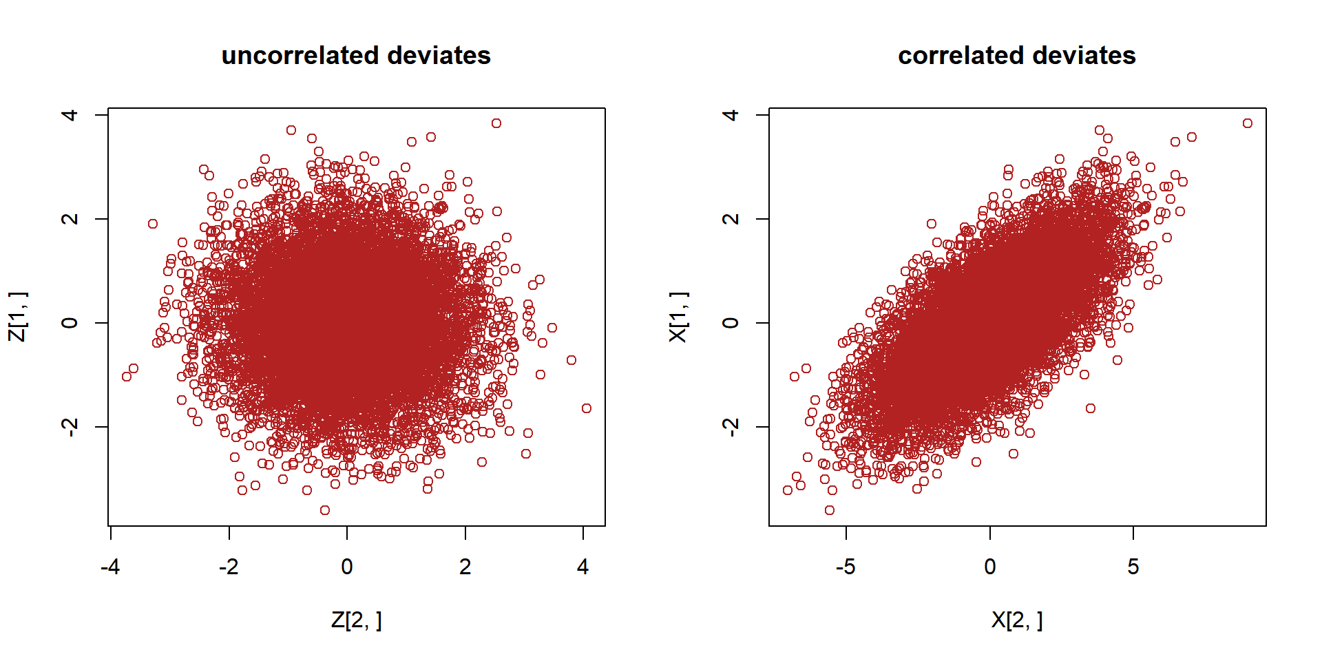
OMEGA <- matrix(c(1, 0.7, 0.7, 1), nrow = 2)
sigmas <- c(1, 2) # sd_b0, sd_b1
OMEGA [,1] [,2]
[1,] 1.0 0.7
[2,] 0.7 1.0[1] 1 2 [,1] [,2]
[1,] 1 0
[2,] 0 2FW 891
Click here to view presentation online
25 October 2023
\[ \begin{array} \text{y}_{i} \sim \operatorname{N}\left(\mu_{i}, \sigma\right) & \text { [likelihood] } \\ \mu_{i}=\beta_{0[group]}+\beta_{1[group]}x_{1[i]} & \text { [linear model] } \\ \end{array} \]
adapted from McElreath 2023
\[ \begin{array} \text{y}_{i} \sim \operatorname{N}\left(\mu_{i}, \sigma\right) & \text { [likelihood] } \\ \mu_{i}=\beta_{0[group]}+\beta_{1[group]}x_{1[i]} & \text { [linear model] } \\ \end{array} \]
Then comes the matrix of varying intercepts and slopes, with it’s covariance matrix \(\mathbf{\Sigma}\):
adapted from McElreath 2023
\[ \begin{array} \text{y}_{i} \sim \operatorname{N}\left(\mu_{i}, \sigma\right) & \text { [likelihood] } \\ \mu_{i}=\beta_{0[group]}+\beta_{1[group]}x_{1[i]} & \text { [linear model] } \\ \end{array} \]
Then comes the matrix of varying intercepts and slopes, with it’s covariance matrix \(\mathbf{\Sigma}\): \[ \begin{array}{l}\begin{aligned}{\left[\begin{array}{c}\beta_{0_{group}} \\ \beta_{1_{group}}\end{array}\right] } & \sim \operatorname{MVN}\left(\left[\begin{array}{l}\beta_{0} \\ \beta_{1}\end{array}\right], \mathbf{\Sigma}\right) \text { [population of varying effects] }\\ \mathbf{\Sigma} & =\left(\begin{array}{cc}\sigma_{\beta_{0}} & 0 \\ 0 & \sigma_{\beta_{1}}\end{array}\right) \mathbf{\Omega} \left(\begin{array}{cc}\sigma_{\beta_{0}} & 0 \\ 0 & \sigma_{\beta_{1}}\end{array}\right) \text { [construct covariance matrix] } \end{aligned} \end{array} \]
adapted from McElreath 2023
adapted from McElreath 2023
adapted from McElreath 2023
adapted from McElreath 2023
adapted from McElreath 2023
adapted from McElreath 2023
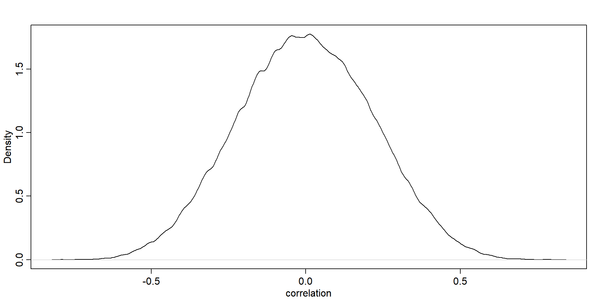
\[ \mathbf{\Omega}=\left(\begin{array}{ll} 1 & \rho \\ \rho & 1 \end{array}\right) \]
adapted from McElreath 2023
\[ \mathbf{\Omega}=\left(\begin{array}{ll} 1 & \rho \\ \rho & 1 \end{array}\right) \]
adapted from McElreath 2023
\[ \mathbf{\Omega}=\left(\begin{array}{ll} 1 & \rho \\ \rho & 1 \end{array}\right) \]
adapted from McElreath 2023
Note that we can take any arbitrary symmetric, positive-definite matrix \(\mathbf{A}\), and factor or decompose it into
\[
\mathbf{A}=\mathbf{L} \mathbf{L}^{T}
\]
where \(\mathbf{L}\) is a lower triangular matrix with real and positive diagonal entries and \(\mathbf{L}^{T}\) is a transpose of \(\mathbf{L}\)
\[ \left[\begin{array}{lll} A_{00} & A_{01} & A_{02} \\ A_{10} & A_{11} & A_{12} \\ A_{20} & A_{21} & A_{22} \end{array}\right]=\left[\begin{array}{lll} L_{00} & 0 & 0 \\ L_{10} & L_{11} & 0 \\ L_{20} & L_{21} & L_{22} \end{array}\right]\left[\begin{array}{ccc} L_{00} & L_{10} & L_{20} \\ 0 & L_{11} & L_{21} \\ 0 & 0 & L_{22} \end{array}\right] \]
\[ \left[\begin{array}{lll} A_{00} & A_{01} & A_{02} \\ A_{10} & A_{11} & A_{12} \\ A_{20} & A_{21} & A_{22} \end{array}\right]=\left[\begin{array}{lll} L_{00} & 0 & 0 \\ L_{10} & L_{11} & 0 \\ L_{20} & L_{21} & L_{22} \end{array}\right]\left[\begin{array}{ccc} L_{00} & L_{10} & L_{20} \\ 0 & L_{11} & L_{21} \\ 0 & 0 & L_{22} \end{array}\right] \]
varying_effects.r scriptsee also Cahill et al. 2020
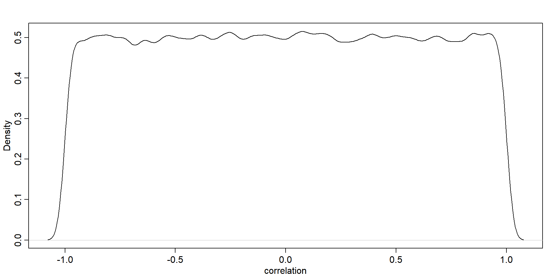
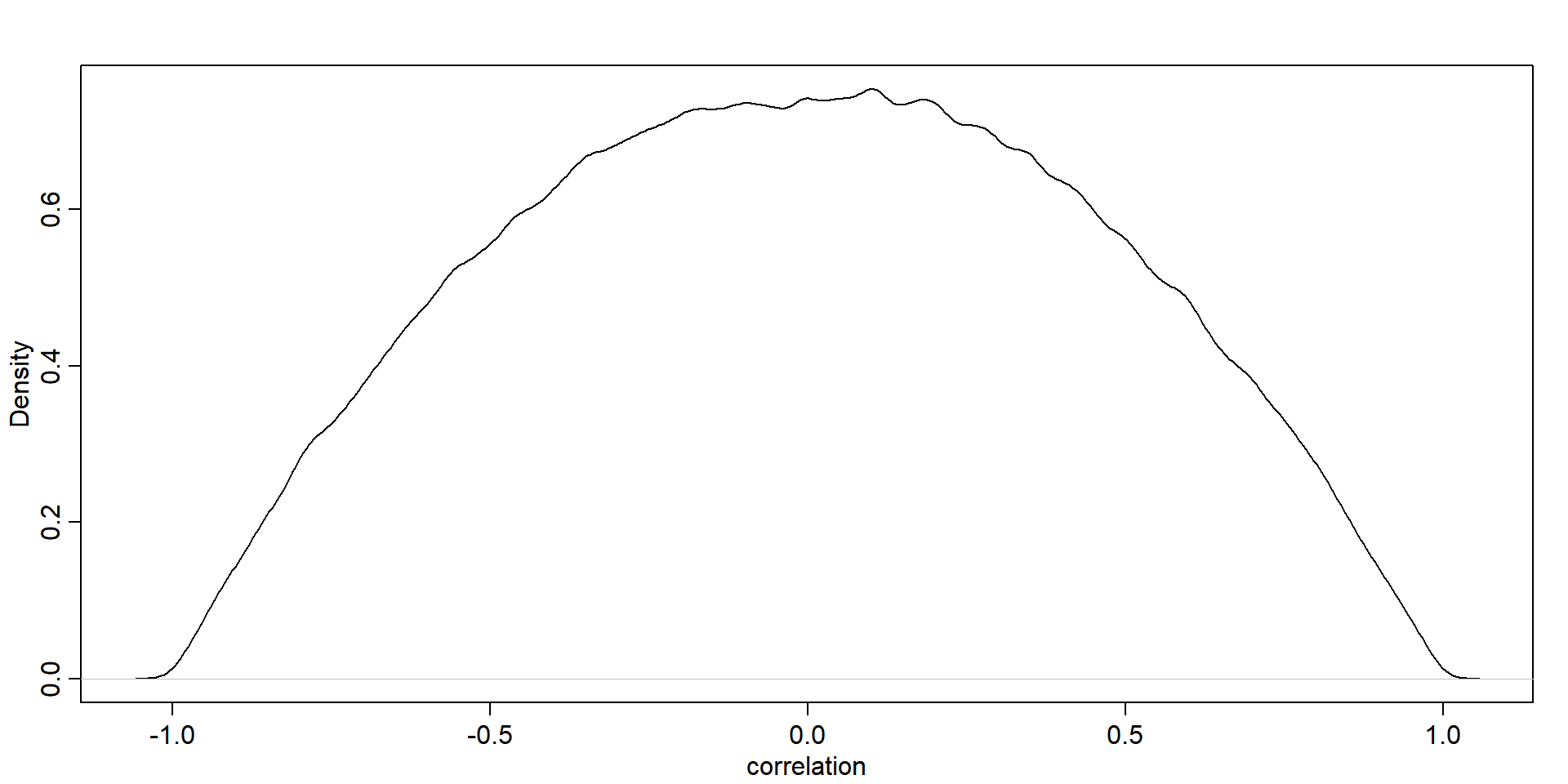
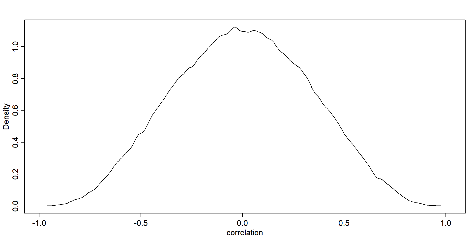
\[ \begin{array}{l}\begin{aligned}\beta_{0} & \sim \operatorname{Normal}(0,25) & \text { [prior for average intercept] }\\ \beta_{1} & \sim \operatorname{Normal}(0,25) & \text { [prior for average slope] } \\ \sigma & \sim \operatorname{Exponential}(0.01) & \text { [prior for stddev within group] }\\ \sigma_{\beta_{0}} & \sim \operatorname{Exponential}(0.01) & \text{[prior stddev among intercepts]}\\ \sigma_{\beta_{1}} & \sim \operatorname{Exponential}(0.01) & \text{[prior stddev among intercepts]}\\ \mathbf{\Omega} & \sim \operatorname{LKJ} \operatorname{corr}(2) & \text{[prior for correlation matrix]} \end{aligned}\\ \end{array} \]
adapted from McElreath 2023
Cahill et al. 2020. A spatial-temporal approach to modeling somatic growth across inland fisheries landscapes. CJFAS.
Gelman, A. and J. Hill. 2007. Data analysis using regression and multilevel/hierarchical models
McElreath 2023. Statistical Rethinking.
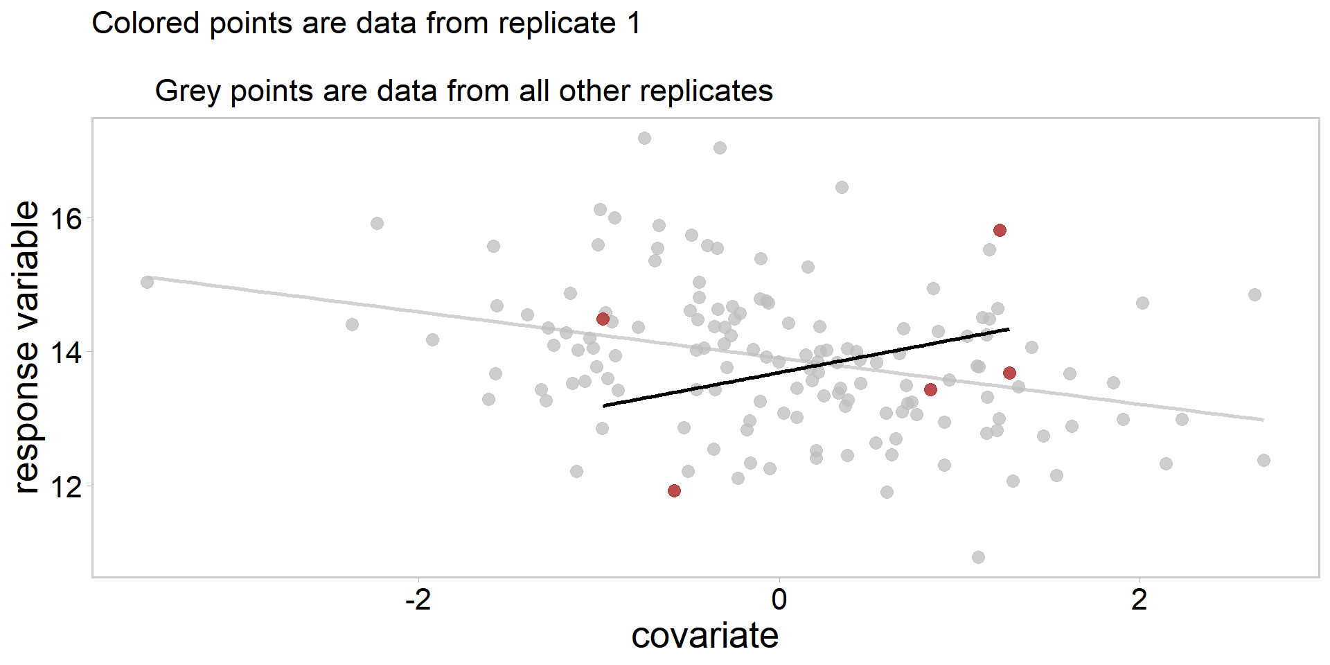
Simpson’s paradox Wikipedia: https://en.wikipedia.org/wiki/Simpson%27s_paradox
https://mlisi.xyz/post/simulating-correlated-variables-with-the-cholesky-factorization/