State-space models
FW 891
Click here to view presentation online
6 November 2023
Purpose
- Goal
- Background
- Some applications and history
- Dynamic linear model and some extensions
- Identifying nonidentifiability
- Future directions and other extensions
- R and Stan demo
A key reference on ecological state space models:
What is a state space model
- State space models are a popular modeling framework for analyzing time-series data
Auger-Methe et al. 2021
What is a state space model
State space models are a popular modeling framework for analyzing time-series data
Useful for modeling population dynamics, metapopulation dynamics, fisheries stock assessments, integrated population models, capture recapture data, animal movement, and biodiversity data
Quite popular because they directly model temporal autocorrelation in a way that helps differentiate process variation vs. observation error.
Auger-Methe et al. 2021
What is a state space model
- A type of hierarchical model
Auger-Methe et al. 2021
What is a state space model
- A type of hierarchical model
- Hierarchical structure accomodates modeling two time series:
Auger-Methe et al. 2021
What is a state space model
- A type of hierarchical model
- Hierarchical structure accomodates modeling two time series:
- A state or process time series that is unobserved and attempts to reflect the true, but hidden, state of nature
- Hierarchical structure accomodates modeling two time series:
Auger-Methe et al. 2021
What is a state space model
- A type of hierarchical model
- Hierarchical structure accomodates modeling two time series:
- A state or process time series that is unobserved and attempts to reflect the true, but hidden, state of nature
- An observation time series that consists of observations related to the state time series
- Hierarchical structure accomodates modeling two time series:
- An example
Auger-Methe et al. 2021
A historical aside
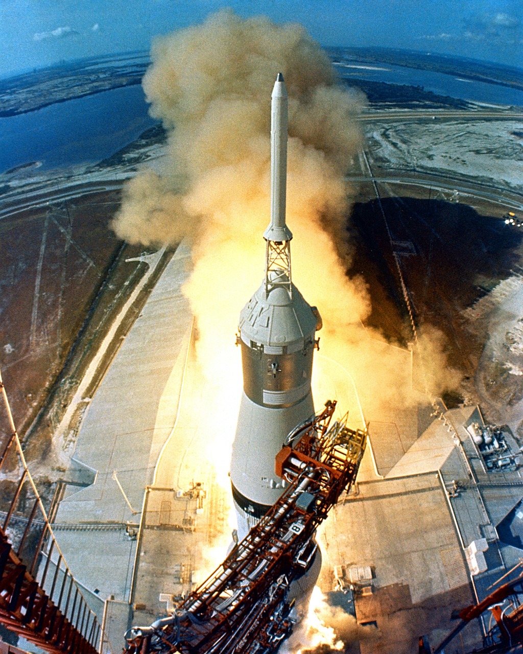
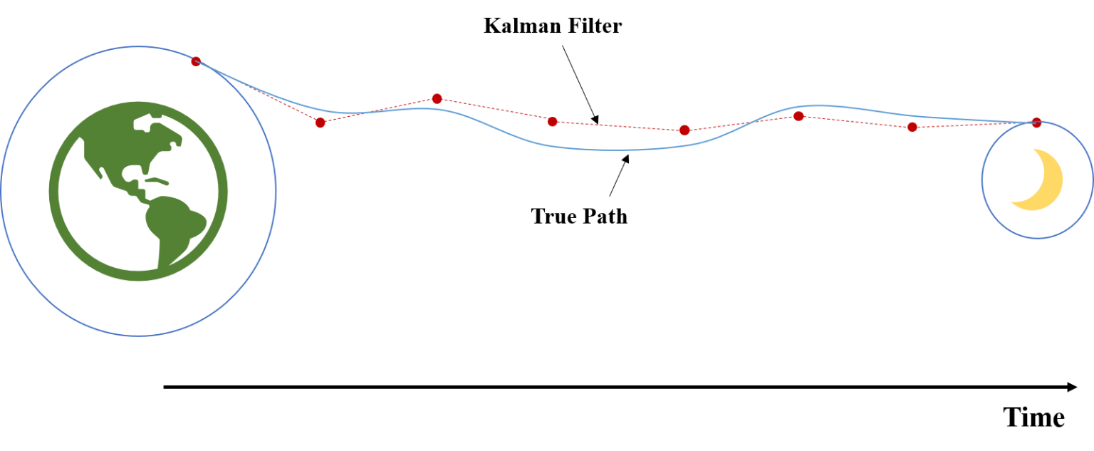
- The Kalman filter
A historical aside
- The Kalman filter
- A mathematical technique that removes “noise” from data
A historical aside
- The Kalman filter
- A mathematical technique that removes “noise” from data
- Used to estimate and control the gradually changing condition of complex systems optimally from incomplete information
A historical aside
- The Kalman filter
- A mathematical technique that removes “noise” from data
- Used to estimate and control the gradually changing condition of complex systems optimally from incomplete information
- Think flight control systems
A historical aside
- The Kalman filter
- A mathematical technique that removes “noise” from data
- Used to estimate and control the gradually changing condition of complex systems optimally from incomplete information
- Think flight control systems
- Importance
A historical aside
- The Kalman filter
- A mathematical technique that removes “noise” from data
- Used to estimate and control the gradually changing condition of complex systems optimally from incomplete information
- Think flight control systems
- Importance
- Remarkably simple and elegant
A historical aside
A historical aside
A historical aside
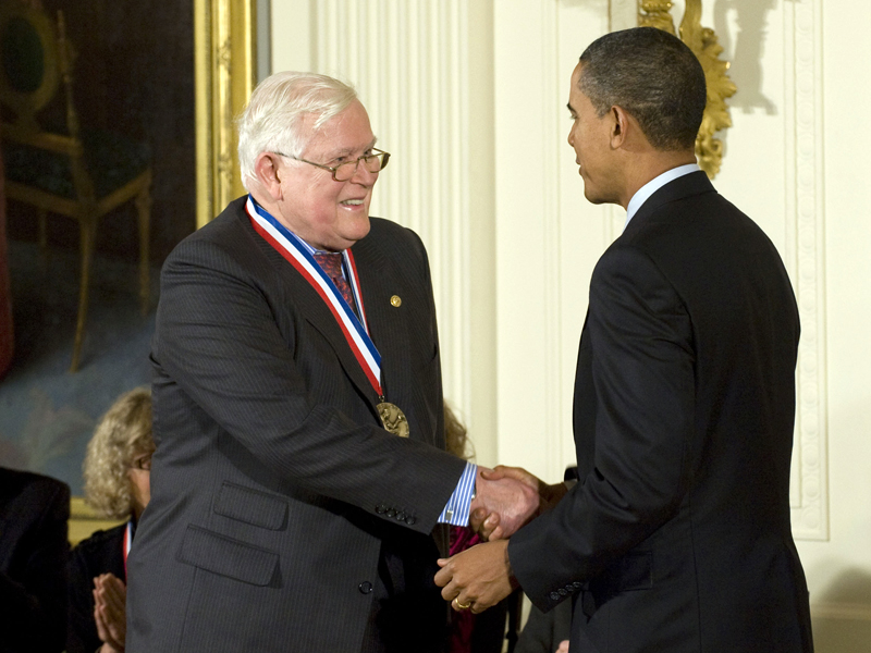
Rudolf Kalman receiving the National Medal of Science from Barack Obama: Photo NAE
Other applications in ecology and resource management?
Other applications in ecology and resource management?
- Hint
Other applications in ecology and resource management?

Walters 1986; Photo: Wikipedia
Other applications in ecology and resource management?

Walters 1986; Photo: Wikipedia
A toy example: normal dynamic linear model
- Time series of univariate observations \(y_{t}\)
- Evenly spaced points in time \(t (t = 1,2,...,T)\)
Auger-Methe et al. 2021
A toy example: normal dynamic linear model
- Time series of univariate observations \(y_{t}\)
- Evenly spaced points in time \(t (t = 1,2,...,T)\)
- Call the time series of states \(z_{t}\)
Auger-Methe et al. 2021
A toy example: normal dynamic linear model
- Time series of univariate observations \(y_{t}\)
- Evenly spaced points in time \(t (t = 1,2,...,T)\)
- Call the time series of states \(z_{t}\)
- Process variance and observation error modeled using Gaussian distributions and both are modeled with linear equations
- This is a normal dynamic linear model
Auger-Methe et al. 2021
The toy example in math:
\[ \begin{array}{c} z_{t}= \alpha + z_{t-1}+\varepsilon_{t}, \quad \varepsilon_{t} \sim \mathrm{N}\left(0, \sigma_{p}^{2}\right), & \color{#E78021}{\text{[process equation]}} \\\\ y_{t}= z_{t}+\eta_{t}, \quad \eta_{t} \sim \mathrm{N}\left(0, \sigma_{o}^{2}\right) . & \color{#8D44AD}{\text{[observation equation]}} \\ \end{array} \]
- The time-series follows a random walk with drift or trend term \(\alpha\)
Auger-Methe et al. 2021
The toy example in math:
\[ \begin{array}{c} z_{t}= \alpha + z_{t-1}+\varepsilon_{t}, \quad \varepsilon_{t} \sim \mathrm{N}\left(0, \sigma_{p}^{2}\right), & \color{#E78021}{\text{[process equation]}}\\\\ y_{t}= z_{t}+\eta_{t}, \quad \eta_{t} \sim \mathrm{N}\left(0, \sigma_{o}^{2}\right) . & \color{#8D44AD}{\text{[observation equation]}} \\ \end{array} \]
- The time-series follows a random walk with drift or trend term \(\alpha\)
- \(\sigma_{p}^{2}\) represents process variance
- \(\sigma_{o}^{2}\) represents obsrvation variance
Auger-Methe et al. 2021
The toy example in math:
\[ \begin{array}{c} z_{t}= \alpha + z_{t-1}+\varepsilon_{t}, \quad \varepsilon_{t} \sim \mathrm{N}\left(0, \sigma_{p}^{2}\right), & \color{#E78021}{\text{[process equation]}} \\\\ y_{t}= z_{t}+\eta_{t}, \quad \eta_{t} \sim \mathrm{N}\left(0, \sigma_{o}^{2}\right) . & \color{#8D44AD}{\text{[observation equation]}} \\ \end{array} \]
- The time-series follows a random walk with drift or trend term \(\alpha\)
- \(\sigma_{p}^{2}\) represents process variance
- \(\sigma_{o}^{2}\) represents obsrvation variance
- \(\varepsilon_{t}\) represent process errors
- \(\eta_{t}\) represent observation errors
Auger-Methe et al. 2021
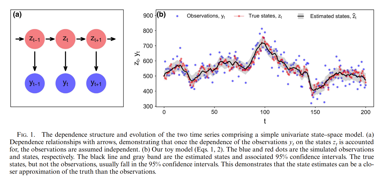
The toy example in pictures
Auger-Methe et al. 2021
Two main assumptions
- State space models (SSMs) assume states evolve as a Markov process, generally as a first order process
Aeberhard et al. 2018; Auger-Methe et al. 2021
Two main assumptions
- State space models (SSMs) assume states evolve as a Markov process, generally as a first order process
- For toy model, this means that the state at time \(t, z_{t}\) depends only on the state at the previous time step \(z_{t-1}\)
- Second, SSMs assume observations are independent of one another after we account for their dependence on the states
- More formally, given some state \(z_{t}\), each observation \(y_{t}\) is conditionally independent of all other observations
- Phrased differently, dependence between observations results from dependence between hidden states \(z_{t}\)
- In a pop dy context, this could be interpretted to mean that \(y_{t}\) values are autocorrelated because the underlying process driving them is autocorrelated through time
Aeberhard et al. 2018; Auger-Methe et al. 2021
The toy example needs one more thing:
\[ \begin{array}{c} z_{t}= \alpha + z_{t-1}+\varepsilon_{t}, \quad \varepsilon_{t} \sim \mathrm{N}\left(0, \sigma_{p}^{2}\right), & \color{#E78021}{\text{[process equation]}} \\\\ y_{t}= z_{t}+\eta_{t}, \quad \eta_{t} \sim \mathrm{N}\left(0, \sigma_{o}^{2}\right) . & \color{#8D44AD}{\text{[observation equation]}} \\ \end{array} \]
- We must define the state at \(z_{t=0}\)
Auger-Methe et al. 2021
The toy example needs one more thing:
\[ \begin{array}{c} z_{t}= \alpha + z_{t-1}+\varepsilon_{t}, \quad \varepsilon_{t} \sim \mathrm{N}\left(0, \sigma_{p}^{2}\right), & \color{#E78021}{\text{[process equation]}} \\\\ y_{t}= z_{t}+\eta_{t}, \quad \eta_{t} \sim \mathrm{N}\left(0, \sigma_{o}^{2}\right) . & \color{#8D44AD}{\text{[observation equation]}} \\ \end{array} \]
- We must define the state at \(z_{t=0}\)
- Typically referred to as the initialization equation
- We’ll set \(z_{t=0} = z_{0}\), where \(z_{0}\) is an estimated parameter
Auger-Methe et al. 2021
Handling nonlinearity
- Our toy example is useful for teaching but rarely helpful in practice
Jamieson and Brooks 2004; Auger-Methe et al. 2021
Handling nonlinearity
- Our toy example is useful for teaching but rarely helpful in practice
- Some useful extensions are
Jamieson and Brooks 2004; Auger-Methe et al. 2021
Handling nonlinearity
- Our toy example is useful for teaching but rarely helpful in practice
- Some useful extensions are
\[ \begin{array}{c} z_{t}=z_{t-1} \exp \left(\beta_{0}+\beta_{1} z_{t-1}+\varepsilon_{t}\right), \quad \varepsilon_{t} \sim \mathrm{N}\left(0, \sigma_{p}^{2}\right) & \color{#E78021}{\text{[process equation]}} \\ y_{t}=z_{t}+\eta_{t}, \quad \eta_{t} \sim \mathrm{N}\left(0, \sigma_{o}^{2}\right) . & \color{#8D44AD}{\text{[observation equation]}} \end{array} \]
- stochastic logistic model
Jamieson and Brooks 2004; Auger-Methe et al. 2021
Handling nonlinearity
- Our toy example is useful for teaching but rarely helpful in practice
- Some useful extensions are
\[ \begin{array}{c} w_{t}=w_{t-1}+\beta_{0}+\beta_{1} \exp \left(w_{t-1}\right)+\varepsilon_{t}, \quad \varepsilon_{t} \sim \mathrm{N}\left(0, \sigma_{p}^{2}\right) & \color{#E78021}{\text{[process eq.]}} \\ y_{t}=\exp \left(w_{t}\right)+\eta_{t}, \quad \eta_{t} \sim \mathrm{N}\left(0, \sigma_{o}^{2}\right) & \color{#8D44AD}{\text{[observation eq.]}} \\ \text{where } w_{t} = log(z_{t}) \\ \end{array} \]
- playing with math and modeling population on logarithmic scale
Jamieson and Brooks 2004; Auger-Methe et al. 2021
Handling nonlinearity
- Our toy example is useful for teaching but rarely helpful in practice
- Some useful extensions are
\[ \begin{array}{c} z_{t}=z_{t-1} \exp \left(\beta_{0}+\beta_{1} \log \left(z_{t-1}\right)+\varepsilon_{t}\right), \quad \varepsilon_{t} \sim \mathrm{N}\left(0, \sigma_{p}^{2}\right) & \color{#E78021}{\text{[process eq.]}} \\ \end{array} \]
- Gompertz model, which assumes that per-unit-abundance growth rate depends on log abundance
Jamieson and Brooks 2004; Auger-Methe et al. 2021
Handling nonlinearity
- Our toy example is useful for teaching but rarely helpful in practice
- Some useful extensions are
\[ \begin{array}{c} w_{t}=\beta_{0}+\left(1+\beta_{1}\right) w_{t-1}+\varepsilon_{t}, \quad \varepsilon_{t} \sim \mathrm{N}\left(0, \sigma_{p}^{2}\right), & \color{#E78021}{\text{[process equation]}} \\ g_{t}=w_{t}+\eta_{t}, \quad \eta_{t} \sim \mathrm{N}\left(0, \sigma_{o}^{2}\right), & \color{#8D44AD}{\text{[observation equation]}} \\ \text{where } w_{t} = log(z_{t}) \text{ and } g_{t} = log(y_{t})\\ \end{array} \]
- Linearized Gompertz model
Jamieson and Brooks 2004; Auger-Methe et al. 2021
What’s the point?

State space models are complex
- e.g., see Thorson et al. 2016
Auger-Methe et al. 2021
State space models are complex
- e.g., see Thorson et al. 2016
- Are there simpler alternatives?
- SSMs superior to simpler models when both the process variance and the observation error are large (e.g., de Valpine and Hastings 2002)
Auger-Methe et al. 2021
State space models are complex
- e.g., see Thorson et al. 2016
- Are there simpler alternatives?
- SSMs superior to simpler models when both the process variance and the observation error are large (e.g., de Valpine and Hastings 2002)
- Many studies have shown that SSMs provided better inference than simpler models
- Should SSMs be the default for many ecological time series?
Auger-Methe et al. 2021
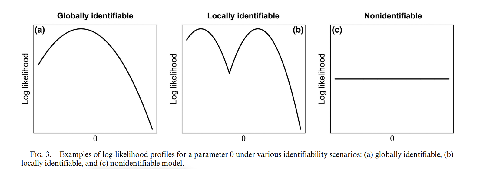
Nonidentifiability

Nonidentifiability
- Identifiability refers to whether there is a unique representation of the model
Auger-Methe et al. 2021
Nonidentifiability
- Identifiability refers to whether there is a unique representation of the model
- Intrinsic vs. extrinsic nonidentifiability
Auger-Methe et al. 2021
Nonidentifiability
- Identifiability refers to whether there is a unique representation of the model
- Intrinsic vs. extrinsic nonidentifiability
- Misusing informed priors may hide identifiability issues
Auger-Methe et al. 2021
Nonidentifiability
- Identifiability refers to whether there is a unique representation of the model
- Intrinsic vs. extrinsic nonidentifiability
- Misusing informed priors may hide identifiability issues
- Diagnostics in the Bayesian framework
Auger-Methe et al. 2021
Nonidentifiability
- Identifiability refers to whether there is a unique representation of the model
- Intrinsic vs. extrinsic nonidentifiability
- Misusing informed priors may hide identifiability issues
- Diagnostics in the Bayesian framework
- Correlation between parameters
- Simulation
- If your model is non-identifiable, parameters are usually biased with large variances
- One should choose priors with great care for SSMs
Auger-Methe et al. 2021
Remedies for nonidentifiability
- Reformulate the model
- Make simplifying assumptions when data are limited
- Estimate measurement errors externally
- Integrate additional data
- Try to use replicated observations
- Match temporal resolution between states and observations
- If one has a data set with locations every 8 h, it would be challenging to estimate behavioral states lasting <16–24 h
Auger-Methe et al. 2021
Wrap up
- SSMs are flexible models for time series that can be used to answer a broad range of ecological questions
- They can be used to model univariate or multivariate time series
- SSMs can be linear or nonlinear, and have discrete or continuous time steps
- Key point:
Auger-Methe et al. 2021
Wrap up
- SSMs are flexible models for time series that can be used to answer a broad range of ecological questions
- They can be used to model univariate or multivariate time series
- SSMs can be linear or nonlinear, and have discrete or continuous time steps
- Key point:
- Recognize that this is a crash course, and there are a great many extensions of SSMs in ecology
Auger-Methe et al. 2021
To the example
References
Aeberhard et al. 2018. Review of state–space models for fisheries science. Annual Review of Statistics and Its Application 5:215–235.
Auger-Methe et al. 2021. A guide to state-space modeling of ecological time series. Ecological Monographs.
de Valpine and Hastings 2002. Fitting population models incorporating process noise and observation error. Ecological Monographs.
Jamieson and Brooks 2004. Density dependence in North American ducks. Animal Biodiversity and Conservation 27:113–128.
Thorson et al. 2016. Joint dynamic species distribution models: a tool for community ordination and spatio-temporal monitoring. Global Ecology and Biogeography 25:1144–1158.
Walters 1986. Adaptive Management of Renewable Resources.