Maximum Likelihood Estimation using RTMB

Lesson 3 - Controlling the search and assessing uncertainty
Click here to view presentation online

Jim Bence

16 December 2024

Outline:

  • Parameterization
  • Fixing parameters
  • Bounding parameters
  • Review and more detail on asymptotic standard errors
  • More than you need to know about the delta method
  • Profile likelihood CIs
  • Self-test simulations and parametric bootstrap

Parameterization - what we want

  • Formal parameters (e.g., what gets sent to nlminb):
    • can legally take values on the entire real number line or are restricted from searching outside bounds (or both)
  • Formal parameters estimates have values on similar scales to one another
  • Formal parameter estimates are not too highly correlated with one another

Functional invariance and parameter transformation

  • Formal (estimated) params transformations of natural params

  • Relies on functional invariance of MLE

    • if NLL(\(\theta\)) = NLL(\(g(\theta)\)) then search on \(\theta\) or on \(g(\theta)\)

    • Example: estimate log_theta and calculate theta=exp(log_theta) inside the NLL function

    • Another example is natural parameters 0<theta<1 or -1<theta<+1 (e.g., correlations)

Logit transformation (for 0-1 or -1 -+1)

\[ \begin{array}{l}b=\operatorname{logit}(a)=\log \left(\frac{a}{1-a}\right) \\a=\operatorname{logit}^{-1}(b)=\frac{1}{1+\exp (-b)}\end{array} \]

  • \(0\leq a \leq1\), \(b\) on real number line, so estimate b then calculate a

  • For \(-1 \leq c \leq +1\) from b (estimate b and calculate c)

    \[ c=2 \operatorname{logit}^{-1}(b)-1=\frac{2}{1+\exp (-b)}-1 \]

Flow when using RTMB

For similar quantities

  • E.g., catchability for different survey gears, or year or location effects
  • One approach: base and offsets
    • Estimate base level (gear, year, location) and offsets
      • Two gears: estimate logqgill and offtrap, logqgill is the log-scale gill net catchability. logqtrap=logqgill+offset
      • for year-effects, estimate YE0, offsets for nyears-1 other years. Then YE[1]=YE0, and (i>1) YE[i]=YE_0+offset[i-1]
  • Alternative is estimate mean and deviations from mean
    • Trickier because for n levels you can estimate the mean and n-1 deviations. The last deviation is calculated.

Forcing parameter order

  • You want theta[1]< theta[2]< theta[3]
    • Estimate theta[1] and two increments
      • theta[2]=theta[1]+inc[1], theta[3]=theta[2]+inc[2]
  • Thought experiment: suppose you are estimating selectivity-at-age and are working with 10 ages so you need sel[i], i=1 to 10.
    • You are willing to assume/define sel[10]=1. You want:
      • 0<=sel[i]<=1
      • sel[i]<=sel[i+1]

My solution

  • Estimate “adjust_par” that determine “adjust” constrained between 0 and 1

  • Loop backwards from i=9 to i=1, with sel[i]=adjust[i]*sel[i+1]

Getting things set up

logit=function(x){
  log(x/(1-x));
}

invlogit=function(x){
  1/(1+exp(-x));
}

# tr_adjust might be starting values of transformed adjusts
tradjust=rep(logit(.9),9);
tradjust;
[1] 2.197225 2.197225 2.197225 2.197225 2.197225 2.197225 2.197225 2.197225
[9] 2.197225

Code like this inside NLL function

adjust = invlogit(tradjust);
sel=rep(NA,10);
sel[10] = 1;
for(i in 1:9){
  sel[10-i] = adjust[10-i]*sel[10-i+1]
}
sel
 [1] 0.3874205 0.4304672 0.4782969 0.5314410 0.5904900 0.6561000 0.7290000
 [8] 0.8100000 0.9000000 1.0000000

Bounds

  • You specify these as vectors for lower and upper bounds

  • These are passed to nlminb (so not part of RTMB)

  • Behavior is different than in admb (bound pars will be failed convergence)

  • Code squib

    #create upper and lower bounds

    lower = c(4,-5,-5,0); upper = c(10,1,5,10);

    #fit with bounds, here “…” the usual args

    fit = nlminb(…, upper=upper, lower=lower);

Fixing (not estimating) a parameter

  • We fix parameters using maps

  • You create a map as a named list where parameters you want to fix are included as factors set to missing values

    E.g., if you wanted to fix loglinf:

    gmmap = list(loglinf=factor(NA));

  • The map is passed as an argument to MakeADFun

    obj=MakeADFun(…, map=grmap);

Exercises

  • Modify the vonB program to bound the parameters (bounds in previous example code reasonable values)

  • Modify the vonB program to not estimate log_linf using a map

  • See if you can combine setting bounds and fixing a parameter (hint: fixed par is not in vector nlminb sees)

Uncertainty, basic definitions of expected value, variance, covariance, and correlation

\[ \mathrm{E}[X]=\int_{-\infty}^{\infty} x f(x) d x \]

\[ \text{Var}(X)=E[(X-E[X])^2] \]

\[ \text{Cov}(X,Y)=E[(X-E[X])(Y-E[Y])] \]

\[ \text{Corr}(X,Y)=\text{Cov}(X,Y)/(\sigma_X \sigma_Y) \]

Confidence Intervals (CIs)

  • An interval that might contain the true value of a parameter (or other estimated quantity)

  • The confidence level is the probability that under repeated sampling the interval does contain the true value.

  • E.g., for a 95% CI, it is expected that 95% of intervals constructed in the same way will include the true value being estimated.

Asymptotic variance covariance matrix and Wald confidence intervals

  • The estimated variances for the parameter estimators are the diagonal elements from matrix, SEs are their square roots.

  • A Wald test assumes \(Z=\left(\hat{\theta}-\theta_{0}\right) / SE\) comes from a N(0,1) distribution, so one would expect \(Pr(|Z|>1.96)=0.05\)

    • One would reject \(H_0: \theta = \theta_0\) at the 0.05 level if \(|Z|>1.96\)
  • A Wald CI inverts a Wald test

Wald Confidence Interval

  • A \(100(1-\alpha) \%\) CI is: \(\hat{\theta} \pm \Phi^{-1}(1-\alpha / 2) S E\), \(\Phi\) is the CDF for a N(0,1) distribution, \(\Phi^{-1}\) is the inverse CDF or quantile function for N(0,1)

  • This is based on inverting a Wald test (i.e., find the Z values that just make the Wald test significant)

  • Special case - 95% CI: \(\hat{\theta} \pm 1.96 S E\)

Delta method

  • This is what ADREPORT uses to get variances for derived (non-parameters) quantities.

  • \(\text{Côv}[g(\underline{\theta}), h(\underline{\theta})] \cong \sum_{i} \sum_{j} \operatorname{Côv} \left[\theta_{i}, \theta_{j}\right] \frac{\partial g(\underline{\theta})}{\partial \theta_{i}} \frac{\partial h(\underline{\theta})}{\partial \theta j}\)

    • Formula for variance is just special case of this.
  • Main point is you can approximate variance of any function of parameters based on covariances of parameters and derivatives of function with respect to parameters

  • If you can get Variances (and hence SEs) you can get Wald CIs

Likelihood ratio test

  • Likelihood profile CI based on inverting a Likelihood Ratio test, with test statistic:

\[ \begin{array} LLRT=-2 \log \frac{\sup \left(L(\underline{\theta}), \underline{\theta} \in \underline{\theta_{0}}\right)}{\sup (L(\underline{\theta}), \underline{\theta} \in \underline{\theta})}= \\-2\left[\log \left(\sup \left(L(\underline{\theta}), \underline{\theta} \in \underline{\Theta}_{0}\right)\right)-\log (\sup (L(\underline{\theta}), \underline{\theta} \in \underline{\theta})]\right. \end{array} \]

  • \(LR T \sim X_{\nu}^{2}\) with \(\nu\) df (based on number of restrictions)

  • Of interest here is \(\underline{\theta} \in \underline{\Theta}_{0}\) with one parameter fixed, testing if that focal parameter differs from fixed value.

    • In this case \(\text{crit}=C D F_{X_{1}^{2}}^{-1}(1-\alpha)\)

Steps in Likelihood ratio test for one fixed parameter

  1. Fit the full model and model with one focal parameter fixed, and extract likelihood (or log likelihood) from results and calculate the test statistic.

  2. Find the critical value (it will always be 3.8415 if one parameter is fixed and your test is at the 0.05 level, otherwise use the chi-square quantile function).

  3. Compare the test statistic with crit and declare significant if crit exceeded.

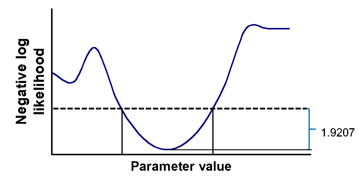
Likelihood profile CI steps

  1. Fit the unrestricted model.  

  2. Repeatedly fit a restricted version of the model with the focal parameter fixed at a range of finely spaced values.

  3. Find the upper and lower values (above and below the point estimate from the unrestricted model) that produce a significant likelihood ratio test.

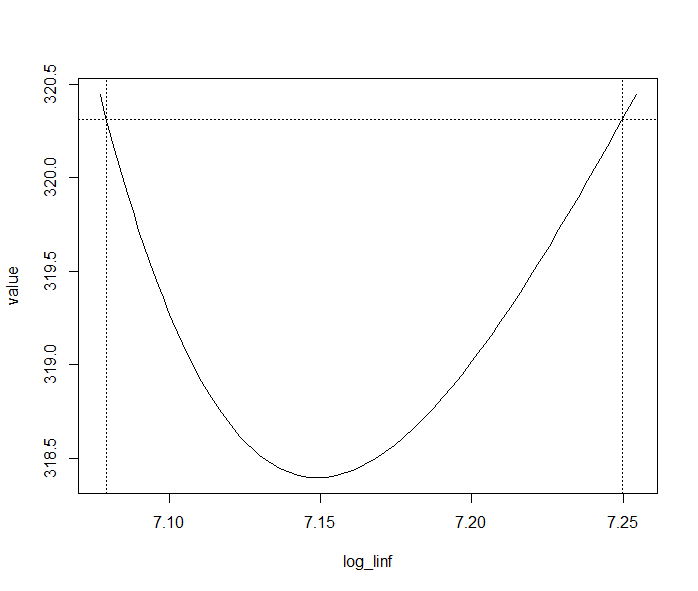
Code to get likelihood profile CI

library(TMB); #load for CI

loglinfprof = tmbprofile(obj,“log_linf”);

confint(loglinfprof);

plot(loglinfprof);

Coding issue

Once you load the TMB package, calls to MakeADFun() do not work unless they explicitly name the RTMB package as in:

RTMB::MakeADFun(…);

Limitation of likelihood profile CIs

  • In TMB for parameters only

  • Some have suggested constraining fit with penalty so desired values of derived quantities could be matched. Theory for this is not fully worked out and its not implemented in TMB.

  • Hence worth exploring simulation approaches (aka parametric bootstrap

    • Simulations of course are for more than CIs

Simulations using RTMB

  • To simulate data from your model you:

    • Mark data you want simulated in your NLL function

      y=OBJ(y);

    • After fitting (or before if you want to simulate from starting values)

      simy=my_obj$simulate()$y

  • Common plan: (1) replace data model was fit to with simulated data, (2) refit the model to this copy and save pertinent results. Repeat 1&2 many times and summarize.

  • I will demo doing one simulation, outline the full simulation procedure, then turn you loose on it.
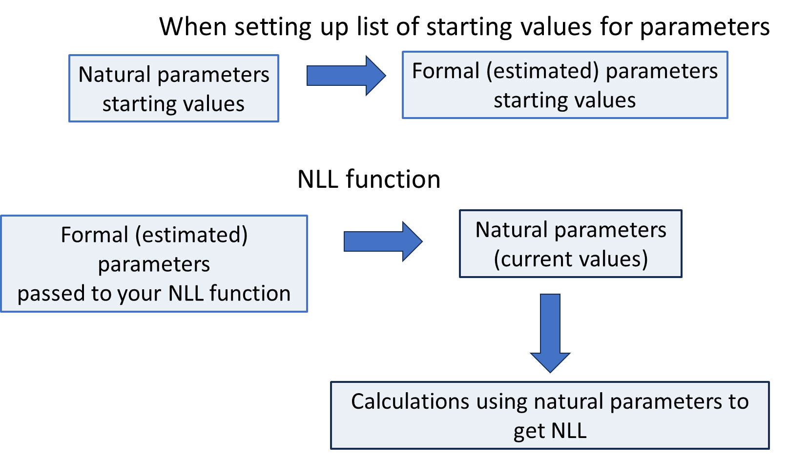
Passing RTMB data

  • MakeADFun expects a function with one argument (named parameter list)
  • It would be nice if we could make both the data and parameters arguments
  • There is way around this - MakeADFun interprets function of function
  • See: musky_vonb_closure.R