Software tools for Maximum Likelihood Estimation
Lesson 4 - Basic random effects in RTMB
Click here to view presentation online
16 December 2024
Outline:
- Overview of purpose of lesson
- What is a random effect
- MLE random effect theory
- The Laplace approximation
- A brief mention, SE in RE models
- Basics of R code to implement random effects
- A first random effects application
Overview/purpose
- learn some basic RE concepts
- learn how to implement a RE model in RTMB
We avoid getting bogged down with the technical details underlying how TMB/RTMB addresses challenges of AD combined with the Laplace transformation. I refer you to Kristensen et al. (2016) an open source pub for more technical material: https://www.jstatsoft.org/article/view/v070i05
What is a random effect
- Random effects seem something like parameters
- But for maximum likelihood estimation parameters cannot be random
- Hence we distinguish (fixed) parameters from random effects
- ultimately (fixed) parameters determine the distributions for REs
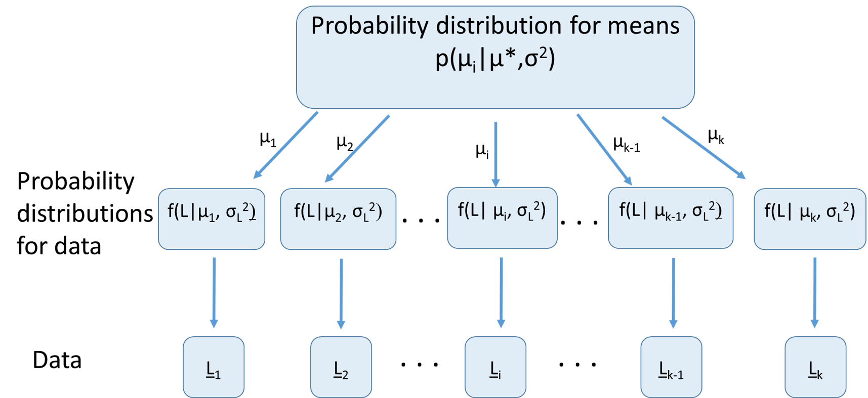
Graphical example of RE model
Advantages of models with REs
Assuming REs come from a common distribution allows information to be shared. E.g., if we know mean length across a number of ponds, we have information about likely mean length in a poorly sampled pond
Sometimes we can analyze data that could not be analyzed with a fixed effect model
- E.g., if an interaction term is viewed as fixed then it requires data for every combination of factors
Inferences can be more general (about the distribution from which the random effects arose)
The strength could become a liability
If dissimilar things are combined.
- You can only share information if there is information to share. E.g., combining 9 bluegill populations and 1 shark population. Does mean length of bluegills tell us much about shark length… Duh!
Too few instances of the random effects to estimate their distributional parameters
MLE Random Effects Theory
The joint likelihood (sometimes aka penalized likelihood)
The marginal (true) likelihood
Why we want to maximize marginal likelihood
The joint likelihood
\[ L(\underline{\theta}, \underline{\gamma} \mid \underline{X})=L\left(\underline{\theta} \mid \underline{\gamma}, \underline{X}\right) p\left(\underline{\gamma} \mid \underline{\theta}\right) \]
Joint likelihood found by taking product of the likelihood conditioned on both RE (\(\underline{\gamma}\)) and data (\(\underline{X}\)) and pdf for random effect conditioned on parameters
Maximizing the joint likelihood is sometimes called penalized likelihood. Basically treats random effects like parameters.
- Substantial limitations and drawbacks to doing this
Marginal likelihood
\[ L(\underline{\theta} \mid \underline{X})=\int_{\underline{\gamma}} L(\underline{\theta}, \underline{\gamma} \mid \underline{X}) d \underline{\gamma}=\int_{\underline{\gamma}} L\left(\underline{\theta} \mid \gamma, \underline{X}\right) p\left(\underline{\gamma} \mid \underline{\theta}\right) d \underline{\gamma} \]
Computationally intensive (integrate over all possible values for the random effects)
Only feasible for complex models in last ~15 years due to software advances
- “smart” AD, implementation of Laplace approximation
Fortunately in RTMB we only have to specify the log of the joint likelihood
Collect together the pieces of log joint likelihood and add them up!
The Laplace approximation
\[ L^{*}(\underline{\theta})=\sqrt{2 \pi^{n}} \operatorname{det}(H(\underline{\theta}))^{-\frac{1}{2}} \exp (-g(\underline{\theta}, \underline{\widehat{\gamma}})) \]
- With \(\underline{\theta}\) fixed at current values, adjust \(\underline\gamma\) to find \(\underline{\widehat{\gamma}}\) that minimizes the neg log joint likelihood \(g(\underline{\theta},\underline{\gamma})\).
- \(H(\underline{\theta})\) is the matrix of second/cross derivatives calculated for the combined vector {\(\underline{\theta},\widehat{\underline{\gamma}}\)}. Written this way to emphasize its function of current value of params
- In the background, during minimization, at each step TMB does an inner minimization to find \(\widehat{\underline{\gamma}}\) so it can apply the Laplace approximation.
Asymptotic standard errors
- Previously we have discussed the delta method used to get asymptotic SEs for derived quantities in fixed effect models. TMB has implemented an adaptation of those methods for estimating SEs for random effects and quantities that involve them, that accounts for uncertainty in the fixed effects (see Skaug and Fournier, 2006: Computational Statistics & Data Analysis, 56, 699–709. doi:10.1016/j.csda.2006.03.005)
What you need to do in R code
- Create a character vector, with the values equaling names of “parameters” you want to be treated as random
- These must match exactly names we used for parameters in our parameter list.
- All declaring a parameter as random asks RTMB to do is integrate it out of the likelihood. You specify the distribution for the random effects in your function you pass to MakeADFun
- Modify your “NLL function” so it returns the negative joint likelihood. This involves subtracting terms equal to log of density for the random effects. This sounds more complicated than it is.
Simple random effects example
Unrealistic example to keep data management dead simple. One observation of length at each age (2-12) for each pond (arranged in a matrix).
fit vonB model for length at age, but now assume asymptotic length (Linf), rather than being a single number, varies among ponds, with the log of Linf for each pond coming from a common normal distribution.
Assume observed length at age normally distributed, with mean generated from the vonB function for that pond (and age), and a common SD shared over ages and ponds.
Before we proceed, what are the parameters (excluding the pond specific Linfs that are now random effects)?
Some exercises
Make logK rather than logLinf a random effect (so now just one logLinf not random)
Estimate logLinf for each pond as a fixed effect rather than a random effect
AIC is calculated as 2k-2*NLL, where k is the number of estimated parameters and NLL is the true (marginal) likelihood. See if you can figure out how to calculate this.