2-02: DataFrame Modifications
0.1 To-do
1 Purpose
Using string manipulations on columns within a data frame
Add, remove, and reorder columns in a data frame
2 Material
The script for this lesson is here
The Lansing2016Noaa.csv is here
3 A larger data frame
For this lesson we are going to use weather data for Lansing, Michigan for all of 2016. The weather data comes from NCDC/NOAA.
To open the data:
weatherData = read.csv(file="data/Lansing2016NOAA.csv",
sep=",",
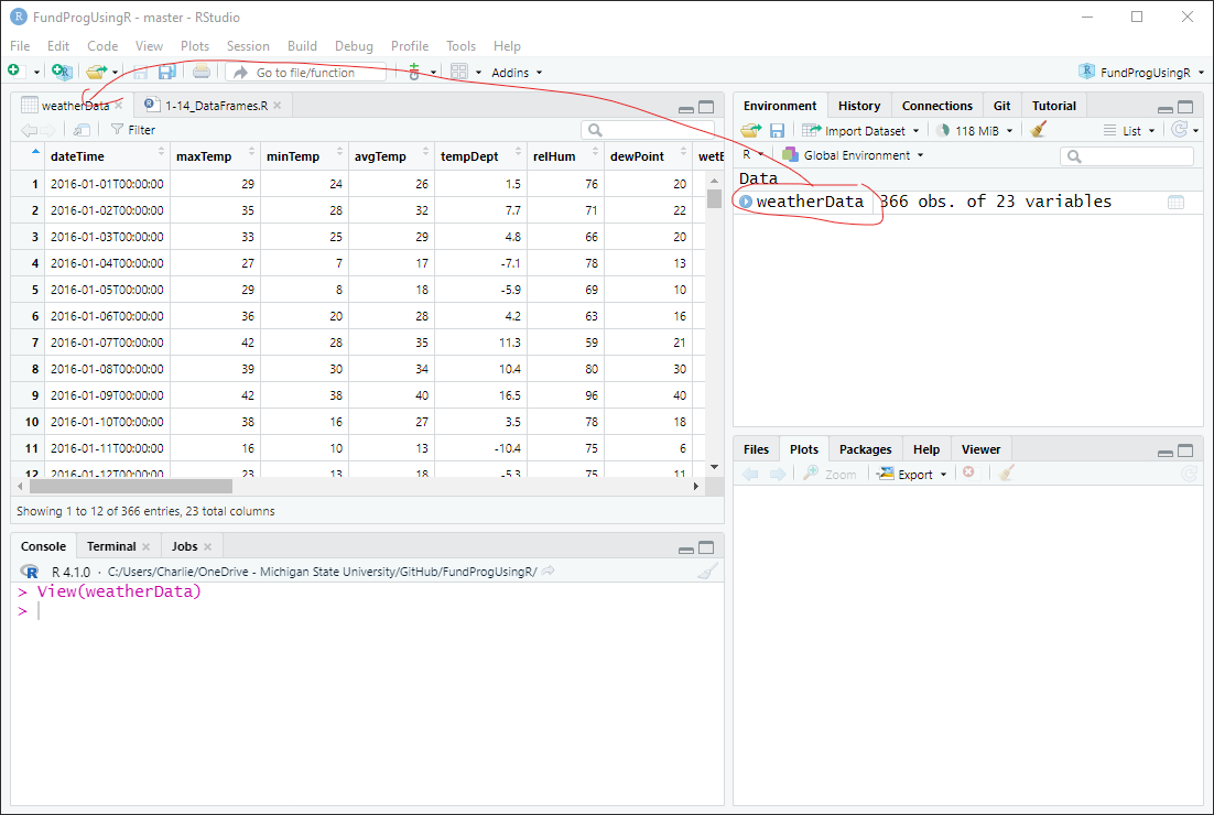
header=TRUE);In the Environment, you can see that weatherData consists of 366 observations (366 days – it was a leap year) of 23 variables. In other words there are 23 different weather variables in the data (columns) for each of the 366 days (rows).
weatherData: 366 obs. of 23 variablesIf we double-click on weatherData in the Environment, we can look at the data frame in the file viewer section of RStudio:
4 String manipulations
There is extra information in the values of the dateTime column (column 1) that is not needed. We really only need the two-digit month and day, which is the 6th through the 10th characters of each dateTime value:
2016-01-02T00:00:00
2016-01-14T00:00:00
2016-01-26T00:00:00
4.1 Substrings
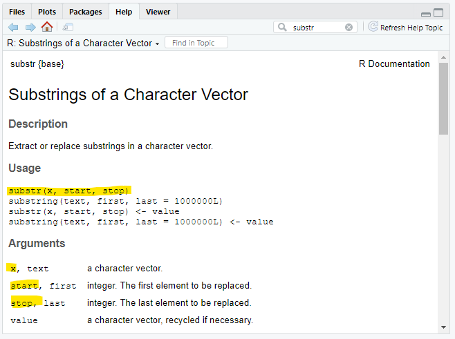
We can use the function substr() to subset, or pull out, a portion of the string’s value.
note: substr() and substring() are practically the same when working with a single string
substr() has three arguments that we need to assign value to:
x: the values that we want to subset (the dateTime column)
start: the position we want the substring to start at (the 6th character)
stop: the position that we want the substring to end at (the 10th character)
dateOnly = substr(x=weatherData$dateTime, start=6, stop=10);This removes the the values between characters 6 and 10 and saves the results to dateOnly.
We can look at the first six values of dateOnly in the Console using head() and the last 6 values using tail():
> head(dateOnly)
[1] "01-01" "01-02" "01-03" "01-04" "01-05" "01-06"
> tail(dateOnly)
[1] "12-26" "12-27" "12-28" "12-29" "12-30" "12-31"
Based on the 12 dates, we can see we have just the 2-digit month and date.
4.2 Pasting values
Let’s say we actually want the year in the column, but we want it at the end.
In other words, we want the date format to be MM-DD-YYYY:
01-02-2016
01-14-2016
01-26-2016
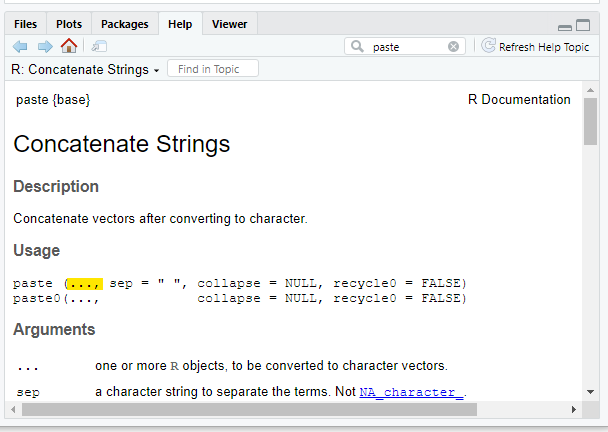
You can use paste() to add (concatenate) string values together.
4.3 three dots ( … ) and arguments
In the Help tab that the first argument in paste() is three dots ( … ). The three dots means that paste() will take any number of objects of any type and try to paste them together.
The three dots represents a pseudo-argument, meaning that for this function, any argument that does not have a name will be assigned to the three dots (i.e., unnamed arguments are objects to be pasted).
This means that you have to use argument names for everything else (e.g., sep, collapse) otherwise paste() will assume the object is to be pasted.
4.4 Using paste()
In this case we want to paste two objects together: the dateOnly vector and the string “-2016” – and we want nothing in between (i.e., nothing separating them):
dateYear = paste(dateOnly, "-2016", sep="");Let’s look at the first ten values in dateYear in the Console:
> dateYear[1:10]
[1] "01-01-2016" "01-02-2016" "01-03-2016" "01-04-2016" "01-05-2016"
[6] "01-06-2016" "01-07-2016" "01-08-2016" "01-09-2016" "01-10-2016"
4.4.1 The sep argument
The sep argument is the character that get placed in between the values being pasted. If you do not put the sep argument in, then sep defaults to one space, meaning an extra space between each object in the paste() – in this case, the date and year:
dateYearDefaultSep = paste(dateOnly, "-2016"); # sep default to " "The results have a space after the date:
> dateYearMistake
01-02 -2016
01-14 -2016
01-26 -2016
Or, you can set sep to some value, and those characters appear between the date and year:
> paste(dateOnly, "-2016", sep="«@!@»")
01-02«@!@»-2016
01-14«@!@»-2016
01-26«@!@»-2016
In general, it is best to set sep=““ (i.e., to nothing) – this gives you more control of the output.
5 Rounding numbers
We have a column, windSpeed, where there are more decimal places than necessary.
Looking at the first ten values in the vector we can see three decimal places are used:
> weatherData$windSpeed[1:10]
[1] 15.539 14.614 9.986 7.742 7.586
[6] 7.601 4.823 6.720 7.294 17.758
One decimal place is probably enough in this case and we can round the values using the round() function:
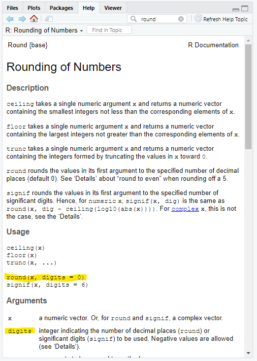
round() has two arguments:
x: the values to round
digits: decimal places to round to
5.1 Using round()
Let’s round windSpeed to one decimal place and save it to the vector windSpeedRounded:
windSpeedRounded = round(weatherData$windSpeed, digits=1);And look at 10 values in windSpeedRounded to make sure it worked (this time I’ll look at values 40-49):
> windSpeedRounded[40:49]
[1] 12.9 13.8 8.9 14.5 9.5 8.1 6.9 3.8 5.9
[10] 10.7In the Console, we are looking at values 40-49 in windSpeedRounded where [1] and the [10] reflects the index value of the output So, value [1] is windSpeedRounded[40], value [2] is windSpeedRounded[41], through value [10] which is windSpeedRounded[49]. Extension: Index values in output
6 Adding vectors to the data frame
We have created two new vectors: dateYear and windSpeedRounded, and we want add them both to the weatherData data frame. There are two ways to add a vector to a data frame:
add a new column
overwrite an existing column.
First, we will make a copy of weatherData called weatherData2. We will be creating multiple copies of weatherData so that we can see the progress of the data frames in the Environment tab. You could just manipulate the original weatherData data frame.
# copy the original data frame
weatherData2 = weatherData;
6.1 Adding a new column
Let’s add the dateYear vector to the data frame to a column called dateYear:
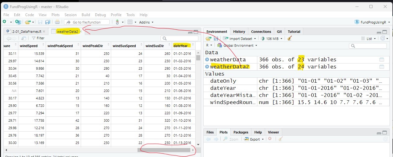
weatherData2$dateYear = dateYear;Since there was no dateYear column in weatherData2, the above code ads a column called dateYear to the end of the data frame and populates it with the values in the vector dateYear. Note that weatherData2 now has one more column (24) than weatherData (23).
Double-click on weatherData2 in the Environment tab and scroll to the end to see the new dateYear column:
6.2 Overwriting a column
When you use a column name that does not currently exist (e.g., dateYear), R will create a new column with that name. If you use a column name that already exists (e.g., windSpeed), then R will overwrite the column with the values in the vector.
We are going to put the windSpeedRounded vector in the weatherData2 data frame, but this time we are going to overwrite the windSpeed column:
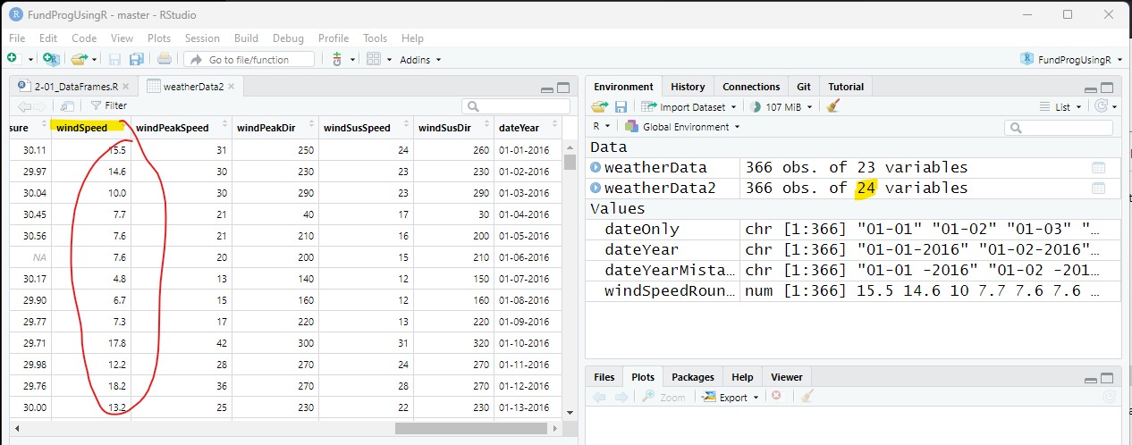
weatherData2$windSpeed = windSpeedRounded;Now the values in the windSpeed column reflect the rounded values from windSpeedRounded and there are still 24 columns:
7 Deleting columns from a data frame
The easiest way to delete a column from a data frame is just to set the column to NULL.
We will create another copy of weatherData:
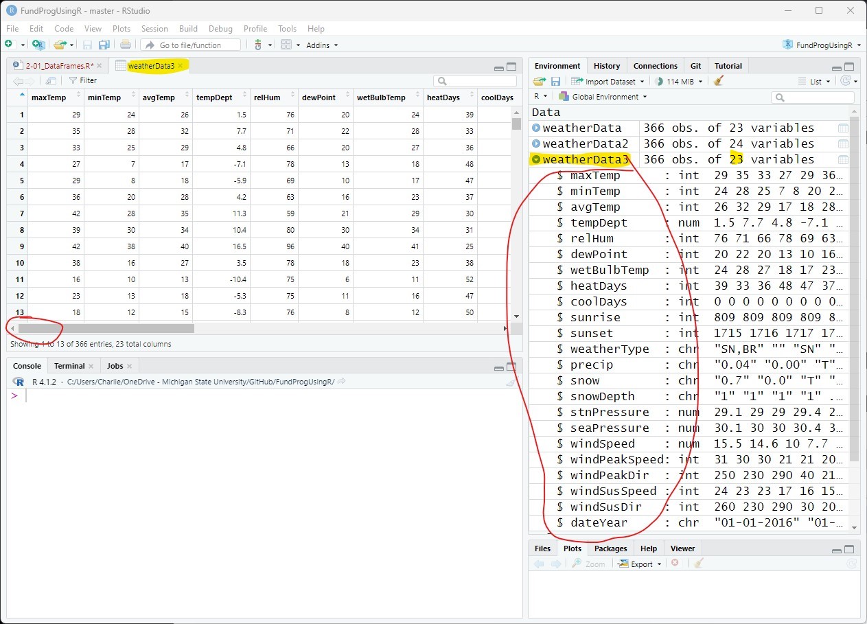
weatherData3 = weatherData2;And remove the dateTime column from weatherData3 by setting it to NULL:
weatherData3$dateTime = NULL; The dateTime column, which was the first column in the data frame, has been removed and the number of columns has dropped by 1 (from 24 to 23):
7.1 Alternate ways to delete columns
You can also use the within() function to remove columns.
Using within() to remove the dateTime column:
# Within weatherData, remove the column dateTime
weatherData3 = within(weatherData, rm(dateTime));
The advantage to this method, is that you can delete multiple columns at a time:
weatherData3 = within(weatherData, rm(maxTemp, minTemp, avgTemp));8 Moving columns
We will make another copy of weatherData here:
weatherData4 = weatherData3;There is no great way to move data frame columns around in R because you cannot just say “move column X to position Y”. Instead, you need to recreate the whole column order of the data frame to reflect the new position of every column – taking care to include every column.
So, let’s say we want to move the dateYear column we created earlier (Section 6.1) from the end of the data frame to the beginning. We essentially need to recreate the 23 columns starting with dateYear first and then have the other 22 columns follow dateYear.
8.1 using sequences to create the column order
Luckily, we do not have to write out all 23 column names because we can use sequences to refer to multiple columns:
# Move the last column (dateYear) to the beginning:
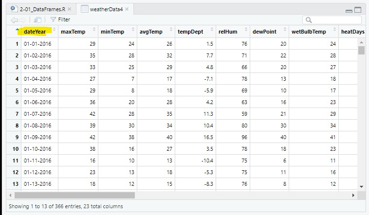
weatherData4 = subset(weatherData2, select=c(dateYear, «maxTemp:windSusDir»));( : ) is the sequence operator and it says to take all the columns in between (and inclusive of) maxTemp and windSusDir. Since maxTemp was the first column and windSusDir was the second to last column (the last being dateYear), this basically says all other columns except dateYear.
So, select=c(dateYear, maxTemp:windSusDir)) says to order the columns with dateYear first and every other column after that.
8.2 A more complex moving example
We will create one last data frame:
weatherData5 = weatherData4;It is trickier to move columns in the middle because you need to keep track of all the other columns.
Let’s says we want to move heatDays and coolDays right after tempDept. These are all columns in the middle of the data frame so you need to break the columns up more to order them the way you want.
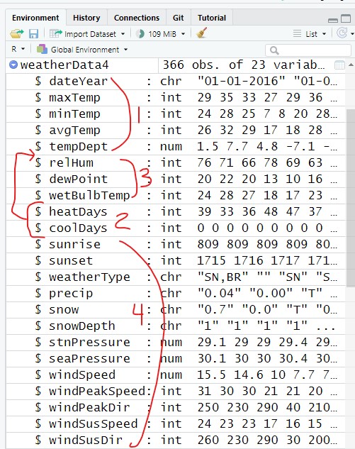
Moving heatDays and coolDays after tempDept creates 4 separate column sequences (Figure 10):
dateYear:tempDept
heatDays:coolDays
relHum:wetBulbTemp
sunrise:windSusDir
8.3 Multiple column sequences
The column sequences above get used in the select argument:
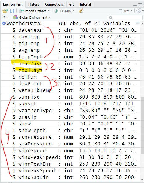
  weatherData5 = subset(weatherData5, select=c(dateYear:tempDept,
                                               heatDays:coolDays,
                                               relHum:wetBulbTemp,
                                               sunrise:windSusDir));
And now we have the reordered columns:
9 Saving the data frame to a CSV file
We are going to use the weatherData5 data frame in the next lesson, so let’s save it to a CSV file.
Quite often, people just call write.csv(), pass in the data frame and the file name to save it to:
write.csv(weatherData5, file="data/Lansing2016Noaa-2-bad.csv"); The above code will add an extra column populated by the row numbers. This is because, by default, write.csv() assumes the row numbers are row names.
To stop write.csv() from assuming the row numbers are row names, we need to set the argument row.names to FALSE:
write.csv(weatherData5, file="data/Lansing2016Noaa-2.csv",
          row.names = FALSE);
In the next lesson, we will open both of these CSV files and look at the difference.
10 Application
A) Save the data from Lansing2016NOAA.csv to a data frame named weatherData_app.
B) Reorder weatherData_app to put all five of the wind columns immediately after the temperature columns.
C) Remove the heatDays and coolDays columns from weatherData_app
D) Using substrings, create a dateTimeNew vector that has the dates in this format: 2-digit date, 2-digit month, 2-digit year.
So, April, 20th 2016 would be 20-04-16
Save dateTimeNew to a column in weatherData_app
Move dateTimeNew to the second column in weatherData_app (do not remove the original dateTime column)
E) Change tempDept in weatherData_app to 2 significant digits – do not use round()
The function for significant digits can be found in the Help for round()
You are overwriting the tempDept column
Save the script as app2-02.r in your scripts folder and email your Project Folder to Charlie Belinsky at belinsky@msu.edu.
Instructions for zipping the Project Folder are here.
If you have any questions regarding this application, feel free to email them to Charlie Belinsky at belinsky@msu.edu.
10.1 Questions to answer
Answer the following in comments inside your application script:
What was your level of comfort with the lesson/application?
What areas of the lesson/application confused or still confuses you?
What are some things you would like to know more about that is related to, but not covered in, this lesson?
11 Extension: Index values in output
Let’s take a closer look at how the index values work in the Console output.
We are going to take a subset of the vector dateYear that goes backwards and only gives at every sixth value.
So, the subset will go: Dec 31, Dec 25, Dec 19, Dec 13…
First, let’s create the sequence:
start at the last value (from = 366)
ends at the first value (to = 1)
moves backwards 6 values each time (by = -6)
> seq(from=366, to=1, by=-6)
 [1] 366 360 354 348 342 336 330 324 318 312 306 300 294 288 282 276 270
[18] 264 258 252 246 240 234 228 222 216 210 204 198 192 186 180 174 168
[35] 162 156 150 144 138 132 126 120 114 108 102  96  90  84  78  72  66
[52]  60  54  48  42  36  30  24  18  12   6
The output has 61 values (366 / 6 = 61). The first value is 366, the 18th value is 264, the 52nd value is 60, and the 61st value is 6.
When we use the sequence to subset dateYear, we also get 61 values, representing the 61 dates on the 61 rows indexed:
> dateYear[seq(from=366, to=1, by=-6)]
 [1] "12-31-2016" "12-25-2016" "12-19-2016" "12-13-2016" "12-07-2016" "12-01-2016"
 [7] "11-25-2016" "11-19-2016" "11-13-2016" "11-07-2016" "11-01-2016" "10-26-2016"
[13] "10-20-2016" "10-14-2016" "10-08-2016" "10-02-2016" "09-26-2016" "09-20-2016"
[19] "09-14-2016" "09-08-2016" "09-02-2016" "08-27-2016" "08-21-2016" "08-15-2016"
[25] "08-09-2016" "08-03-2016" "07-28-2016" "07-22-2016" "07-16-2016" "07-10-2016"
[31] "07-04-2016" "06-28-2016" "06-22-2016" "06-16-2016" "06-10-2016" "06-04-2016"
[37] "05-29-2016" "05-23-2016" "05-17-2016" "05-11-2016" "05-05-2016" "04-29-2016"
[43] "04-23-2016" "04-17-2016" "04-11-2016" "04-05-2016" "03-30-2016" "03-24-2016"
[49] "03-18-2016" "03-12-2016" "03-06-2016" "02-29-2016" "02-23-2016" "02-17-2016"
[55] "02-11-2016" "02-05-2016" "01-30-2016" "01-24-2016" "01-18-2016" "01-12-2016"
[61] "01-06-2016"
Again, the index values in square brackets is just given you the index value of the first value on the row. So, 12-31 is the first value, 12-01 is the 5th value, 11-25 is the 7th value, and 01-06 is the 61st value.