2-10: Statistical Tests
0.1 to-do
- more on the difference between rdata and rds files
1 Purpose
Opening , and using data from, rdata files
Use t-tests and ANOVAS
demonstrate subsetting methods
plot and calculate a linear regresion
2 Script and data for this lesson
The script for the lesson is here
The List file created in the last lesson: tempDFs.rdata
3 Reading in the rdata file (List from last lesson)
In previous lesson, we opened up a CSV file and saved the data to a data frame using read.csv(). In this lesson, we are going to use some of the data frames created in the last lesson – data frames that were saved to a rdata file in the data folder of our project.
From last lesson:
# save(temperatureDFs, file = "data/tempDFs.rdata");Extension: rds and rdata files
Now, let’s open up the file using load():
load(file = "data/tempDFs.rdata");Inside the rdata file is a List object, temperatureDFs, with four data frames. In the next couple lessons we will be dealing a lot more with navigating and creating List objects. For now, a List object is a container for other object (like data frames). load() takes the objects from the rdata file and puts in the Environment:
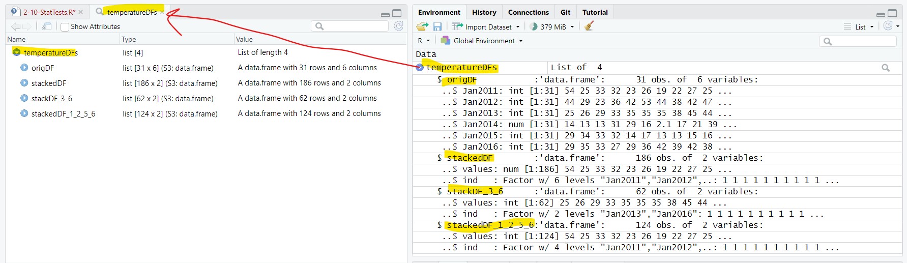
3.1 Extracting the data frames
The data frames inside the List can be extracted just like a column can be extracted from a data frame. Let’s extract the four data frame using the ( $ ) subset operator:
lansJanTempsDF = temperatureDFs$origDF;
stackedDF = temperatureDFs$stackedDF;
stackedDF2 = temperatureDFs$stackDF_3_6;
stackedDF3 = temperatureDFs$stackedDF_1_2_5_6;
This put the data frames directly in the Environment:
⮞ lansJanTempsDF:   31 obs. of 6 variables
⮞ stackedDF:        186 obs. of 2 variables
⮞ stackedDF2:       62 obs. of 2 variables
⮞ stackedDF3:       124 obs. of 2 variables
4 t-tests
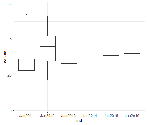
In the last lesson, we created line plot and box plot to display the temperature data. Let’s be more formal about analyzing the data and do a two-sample t-test. In statistics, a two-sample t-test is used to determine if there is evidence that the means from two groups of values are different. In this case, we are asking if the columns (years) in the matrix, are statistically different.
4.1 first t-test on columns that do not look similar
We are going to compare the means from January 2012 (column 2) and January 2014 (column 4). – two columns that visually (Figure 2) do not look similar at all. To perform a t-test between these two years, we call the function t.test() and use the arguments x and y. x and y are set to the two columns we are comparing using the subset operator ( $ ).
tTest1 = t.test(x=lansJanTempsDF$Jan2012, y=lansJanTempsDF$Jan2014);In the Environment tab, tTest1 is labelled as a “List of 10”. There is a lot of information in that List and we will dig more into this later. For now, we can get a helpful summary using the function print() and passing it the results of the t-test:
print(tTest1);> print(tTest1);
Welch Two Sample t-test
data: lansJanTempsDF$Jan2012 and lansJanTempsDF$Jan2014
t = 4.7784, df = 59.561, p-value = «1.195e-05»
alternative hypothesis: true difference in means is not equal to 0
95 percent confidence interval:
«7.212138 17.600765»
sample estimates:
mean of x mean of y
«35.77419 23.36774»In the summary of the t-test it is stated that
The mean of x (Jan 2012) is 35.77419 and the mean of y (Jan 2014) is 23.36774
If the “experiment” could be repeated, we would expect to see a difference of this size between the means 0.001195% of the time (from the p-value of 1.195e-05 or 0.00001195)
We are 95% sure that the means of x and y have a difference between 7.212138 and 17.600765
- So, 0, or no difference is not within our confidence interval
In this case, we would reject the null hypothesis that the means of x and y are equal – in other words, January 2012 and 2014 temperatures are statistically different.
4.2 second t-test on columns that do look similar
We will do a second t-test between years that do look as visually similar (Figure 2) – 2013 (column 3) and 2016 (column 6):
tTest2 = t.test(x=lansJanTempsDF[,3], y=lansJanTempsDF[,6]);And, let’s summarize the results of the t-test in the Console tab:
>   print(tTest2);

    Welch Two Sample t-test

data:  lansJanTempsDF[, 3] and lansJanTempsDF[, 6]
t = 0.88083, df = 53.993, p-value = «0.3823»
alternative hypothesis: true difference in means is not equal to 0
95 percent confidence interval:
 «-3.087414  7.926124»
sample estimates:
mean of x mean of y
«34.16129 31.74194» In the summary of the t-test it is stated that
The mean of x (Jan 2013) is 34.16129 and the mean of y (Jan 2016) is 31.74194
If the “experiment” could be repeated, we would expect to see a difference of this size between the means 38.23% of the time (from the p-value of 0.3823)
We are 95% sure that the means of x and y have a difference between -3.087414 and 7.926124
- So, 0, or no difference is within our confidence interval
In this case, we would not reject the null hypothesis that the means of x and y are equal – in other words, January 2013 and 2016 temperatures are statistically similar.
4.3 Seven ways to subset columns in a Data Frame
For tTest1 an tTest2, we used 2 different methods for subsetting a column in a dataframe. There are actually seven ways to subset a column in a data frame and they all produce the same result.
This is because there are four different operators that you can use to subset a data frame and for three of the operators you can use numbers or names:
$: dollar sign operator (note: this is the only operator where you cannot use a number)
[ ,]: row/column operator (note: this is the only subset operator that works for a matrix)
[ ] : single bracket operator
[[ ]]: double bracket operator
1) The row-column operator [ , ] using column numbers (also works on a matrix):
tTest2a = t.test(x=lansJanTempsDF[,2], y=lansJanTempsDF[,4]);2) The row-column operator [ , ] using column names (also works on a matrix):
tTest2b = t.test(x=lansJanTempsDF[,"Jan2012"], y=lansJanTempsDF[,"Jan2014"]);3) The single bracket operator [ ] using column numbers:
tTest2c = t.test(x=lansJanTempsDF[2], y=lansJanTempsDF[4]);4) The single bracket operator [ ] using column names:
tTest2d = t.test(x=lansJanTempsDF["Jan2012"], y=lansJanTempsDF["Jan2014"]);5) The double bracket operator [[ ]] using column numbers:
tTest2e = t.test(x=lansJanTempsDF[[2]], y=lansJanTempsDF[[4]]);6) The double bracket operator [[ ]] using column names:
tTest2f = t.test(x=lansJanTempsDF[["Jan2012"]], y=lansJanTempsDF[["Jan2014"]]);7) The dollar sign operator $ using column names (you cannot use $ with column numbers):
tTest2g = t.test(x=lansJanTempsDF$Jan2012, y=lansJanTempsDF$Jan2014;4.4 Summary of subset operators
The operators in general (and in order of this author preference):
The $ operator is the most convenient because it requires the least code and RStudio will give you suggestions
The [ , ] operator is the most robust because it is explicit about the two-dimensionality of the data frame, allowing you to subset the rows along with the columns. This is the best choice if you are subsetting rows and columns at the same time
The [[ ]] operator is best used for more complex object like Lists – I generally avoid these when using data frames
The [ ] operator does a different kind of subsetting than the other three operators that will be explored in the next lesson. This author would argue that it is the least useful operator
5 ANOVAs
ANOVAs are similar to t-tests except they generally are used to test the means from three or more groups of data, whereas a t-test can only test the means from two groups. For comparison, we are going to start by using an ANOVA on 2 groups (Jan2013 and Jan2016).
ANOVAs are functionally similar to a t-test but R requires that the data be structured differently before performing an ANOVA. In R, the ANOVA function aov() cannot compare values from different columns like t.test(). Instead aov() compares values within a column grouped by a second column.
In other words, to perform an ANOVA using aov(), you need to use a stacked dataframe and we will use the stacked data frames created in the last lesson and loaded in from the rdata file.
Note: the reason why aov() requires a stacked data frame is largely a legacy issue
5.1 Performing an ANOVA
We will perform an ANOVA on stackedDF2, which contains data from only Jan2013 and Jan2016, to check whether the January temperatures from the two years are likely to be from the same distribution.
To perform an Anova using aov() you need two arguments:
data: the (stacked) data frame that contains the data
- in this case: the stacked data frame stackedDF2
formula: the columns used for the ANOVA in the form: all_values~grouping
- all_values comes from the values column and the grouping comes from the ind column (note: this is similar to an x, y mapping GGPlot except that it is in the form y~x)
Jan13_16_Anova = aov(data=stackedDF2, formula=values~ind);To get the results of the ANOVA you need to print the summary of the Anova:
print(summary(Jan13_16_Anova);Doing this in the Console tab, we get:
>   print(summary(Jan13_16_Anova));
            Df Sum Sq Mean Sq F value Pr(>F)
ind          1     91   90.73   0.776  «0.382»
Residuals 60 7016 116.94 The results of the ANOVA show the probability that the temperatures come from the same distribution is 0.382 (38.2%). This, as expected, is the very close to the same probability (0.3823) that we got from doing the t-test between 2013 and 2016 and means we do not reject the NULL hypothesis that the groups come from the same distribution.
5.2 A Second ANOVA <make into application>
We are going to perform a second ANOVA on the 4 years (2011, 2012, 2015,and 2016) in stackedDF3 created in last lesson.
The Anova call looks almost the same:
Jan4MonthAnova = aov(data=stackedDF3, formula=values~ind);Summarizing the ANOVA in the Console tab:
>   print(summary(Jan4MonthAnova));
             Df Sum Sq Mean Sq F value   Pr(>F)
ind           3   1923   641.0   8.617 «3.17e-05» ***
Residuals   120   8926    74.4
---
Signif. codes:  0 ‘***’ 0.001 ‘**’ 0.01 ‘*’ 0.05 ‘.’ 0.1 ‘ ’ 1
The results of the ANOVA show that the probability of the four sets of January temperatures coming from the same distribution is 3.17e-05, or 0.00317%. In this case, we reject the NULL hypothesis that the groups come from the same distribution.
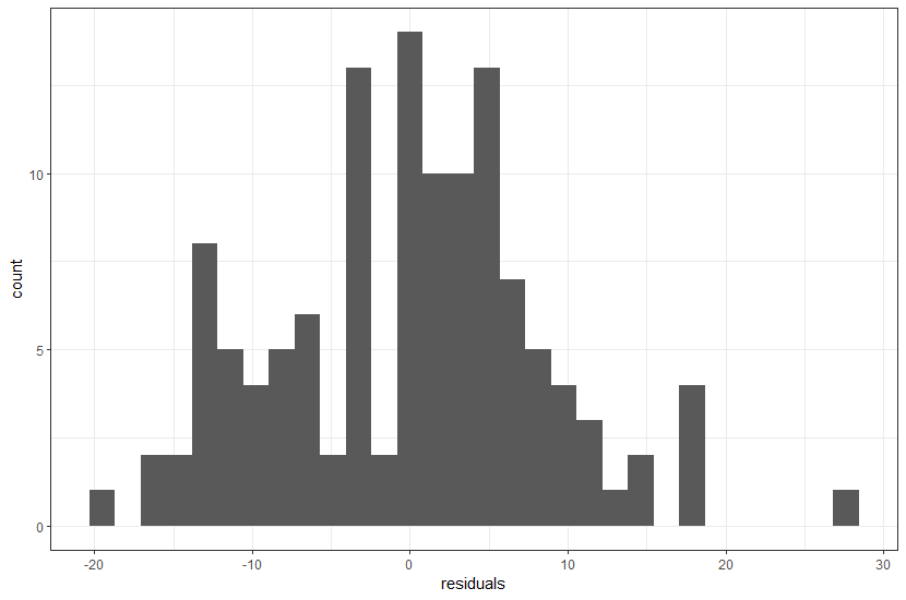
5.3 Residuals: checking for normailty
Lastly, we can perform a histogram on the residuals of the ANOVA to show the we have not violated normality assumptions.
The residuals() function gets the 124 residuals from Jan4MonthAnova:
residuals = residuals(Jan4MonthAnova);residuals: Named num [1:124] 28.387 -0.613 7.387 6.387 ...We can then plot the residuals vector in a histogram by mapping the vector to x (the y-axis is count as does not get mapped):
plot1 = ggplot() +
  geom_histogram(mapping=aes(x=residuals)) +
  theme_bw();
plot(plot1);
… and this histogram looks fairly normal so we probably did not violated the normality assumption.
6 Linear Regression
For linear regressions, we will be using the data from the bigger data set found in Lansing2016Noaa-3.csv:
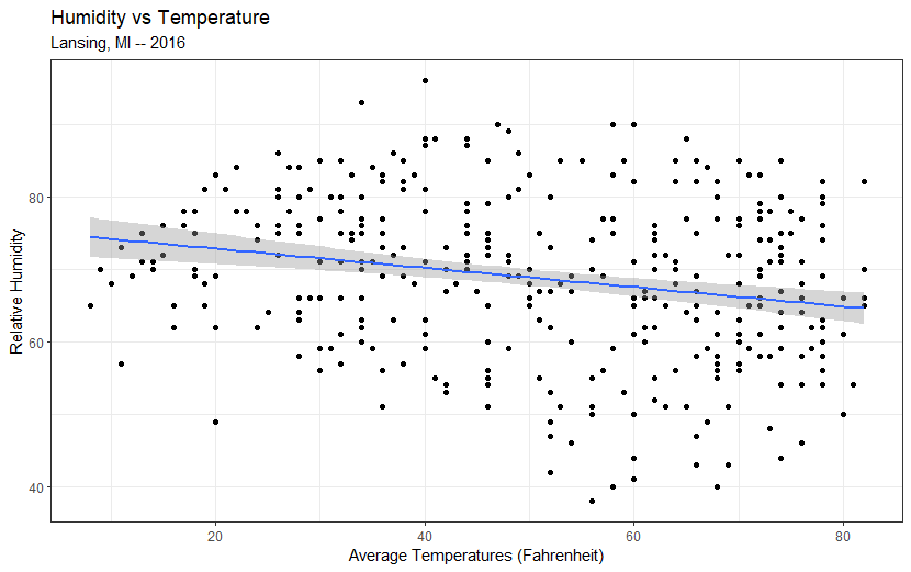
weatherData = read.csv(file="data/Lansing2016Noaa-3.csv");In the GGPlot introductory lesson (2-01), we did a scatterplot of humidity vs. temperature using a geom_point component and added a linear regression using geom_smooth.
plot1 = ggplot(data=weatherData) +
  «geom_point»( mapping=aes( x=avgTemp, y=relHum ) ) +
  «geom_smooth»( mapping=aes( x=avgTemp, y=relHum ),
               method="lm" ) +
  labs( title="Humidity vs Temperature",
        subtitle="Lansing, MI -- 2016",
        x = "Average Temperatures (Fahrenheit)",
        y = "Relative Humidity") +
  theme_bw();
plot(plot1);
The plot looks like this:
6.1 Calculate a linear regression
We can formalize the calculation of the humidity vs. temperature linear regression using lm().
The argument we need to set for lm() is formula and formula is in this form: y ~ x
So, y is the humidity column and x is the temperature column:
tempHumLM = lm( formula = weatherData$relHum ~ weatherData$avgTemp );We can print() the results to the Console and see the intercept is about 75 and the slope is about -0.13:
>   print(tempHumLM);

Call:
lm(formula = weatherData$relHum ~ weatherData$avgTemp)
Coefficients:
        (Intercept)  weatherData$avgTemp
            «75.4863»              «-0.1326»
The results closely match the linear regression in the plot in Figure 7 .
We can get a lot more information using print(summary()):
>   print(summary(tempHumLM));

Call:
lm(formula = weatherData$relHum ~ weatherData$avgTemp)

Residuals:
     Min       1Q   Median       3Q      Max
-30.0624  -7.5984   0.3051   8.2171  25.8165

Coefficients:
                    Estimate Std. Error t value Pr(>|t|)
(Intercept)         «75.48632»    1.61703  46.682  < 2e-16 ***
weatherData$avgTemp «-0.13257»    0.02988  -4.437 1.21e-05 ***
---
Signif. codes:  0 ‘***’ 0.001 ‘**’ 0.01 ‘*’ 0.05 ‘.’ 0.1 ‘ ’ 1

Residual standard error: 10.88 on 364 degrees of freedom
Multiple R-squared:  «0.0513»,    Adjusted R-squared:  0.04869
F-statistic: 19.68 on 1 and 364 DF,  p-value: «1.213e-05»
The slope and intercept are in this summary. The R-squared value tells us that temperature explains about 5.13% (0.0513) of the variance in humidity and the p-value of 1.21e-05 (0.0000121) says we reject the NULL hypothesis that temperature is not a predictor of humidity. In other words, changes in temperature can predict some change in humidity.
7 Application
1) Subset the first 10 values from column 6 of lansJanTempsDF four times using four different methods (Section 4.3).
2) Based on the boxplot of all 6 years ( Figure 2 ), which three years would most likely come form the same distribution (i.e., the ANOVA would not reject the NULL hypothesis).
create a stacked frame with just these three years
perform an ANOVA on the three years
print the result to the Console
3) Using t-tests, find which year’s January temperatures is most statistically similar to the temperatures from January 2014 (other than itself!).
4) Perform four linear models:
stnPressure vs. windSpeed,
stnPressure vs. precipNum
stnPressure vs. avgTemp
stnPressure vs. relHum
5) Using only the linear model from #4 that shows the most correlation:
print the summary to the Console and explain the summary in comments
create a scatterplot of the two variables
place a regression line on the scatterplot
create a histogram of the residuals
Save the script as app2-10.r in your scripts folder and email your Project Folder to Charlie Belinsky at belinsky@msu.edu.
Instructions for zipping the Project Folder are here.
If you have any questions regarding this application, feel free to email them to Charlie Belinsky at belinsky@msu.edu.
7.1 Questions to answer
Answer the following in comments inside your application script:
What was your level of comfort with the lesson/application?
What areas of the lesson/application confused or still confuses you?
What are some things you would like to know more about that is related to, but not covered in, this lesson?
8 Extension: rds and rdata files
In the last lesson, we saved the List object temperatureDFs to two different types of files: rdata and rds.
The two types of files serve a similar purpose: saving objects from your Environment to your Project Folder to be used later. The big difference between the two is how they are later loaded into your Environment.
When you load an rdata file, the objects in the rdata file get loaded directly into you Environment exactly as they previously were (i.e., same name as values). In this case, the List temperatureDFs is directly loaded into the Environment:
load(file = "data/tempDFs.rdata");When you load an rds file, the object in the rds file need to be saved to a variable to get loaded into you Environment. This means the values are the same but the name could be different. In this case, the information from temperatureDFs is save to a variable named tempDFs2:
tempDFs2 = readRDS(file="data/tempDFs.rds");8.1 Pro and cons
RData files are the quick-and-dirty way to save R objects and reload them later. A single .RData file can store multiple objects, and you can even save an entire Environment at once. This is convenient for short-term work, for example restoring your Environment the next morning. However, loading an .RData file restores objects directly into the Environment, which can have unintended consequences: existing objects with the same names will be overwritten. This makes .RData files risky in larger scripts and collaborative settings.
RDS files are the safer and more collaborator-friendly way to save objects. An .rds file stores exactly one object. The file contains the object’s data, but not its name. When loading the file, the user explicitly assigns the object to a variable name of their choosing. This explicit assignment avoids accidental overwrites, and leads to workflows that are easier to reproduce and maintain.