2-03: Data Types and Data Frames
0.1 To-do
1 Purpose
Manipulations of a data frames
Converting a column’s datatype
2 Material
Like last lesson we will fixing some typical issues of columns in a data frame and we will also be manipulating the data frame to reflect the changes
The script for this lesson is here
We will be looking at two data frames in this lesson:
The Lansing2016Noaa-2-bad.csv is here
The Lansing2016Noaa-2.csv is here
3 Extra columns in data frames
We are going to start this lesson by looking at a couple issues that occur when writing a data frame to a CSV file.
In the last lesson we wrote to two CSV files, the first one using all default values for write.csv():
write.csv(weatherData5, file="data/Lansing2016Noaa-2-bad.csv"); # from last lessonLet’s open up this file and see what happened:
badData = read.csv(file="data/Lansing2016NOAA-2-bad.csv",
              sep=",",
              header=TRUE);
After you double-click on badData in the Environment tab, you can see there is an extra column in the data frame at the beginning which has the row numbers in it. This is because, by default, write.csv() will treat the row numbers as a column of data.
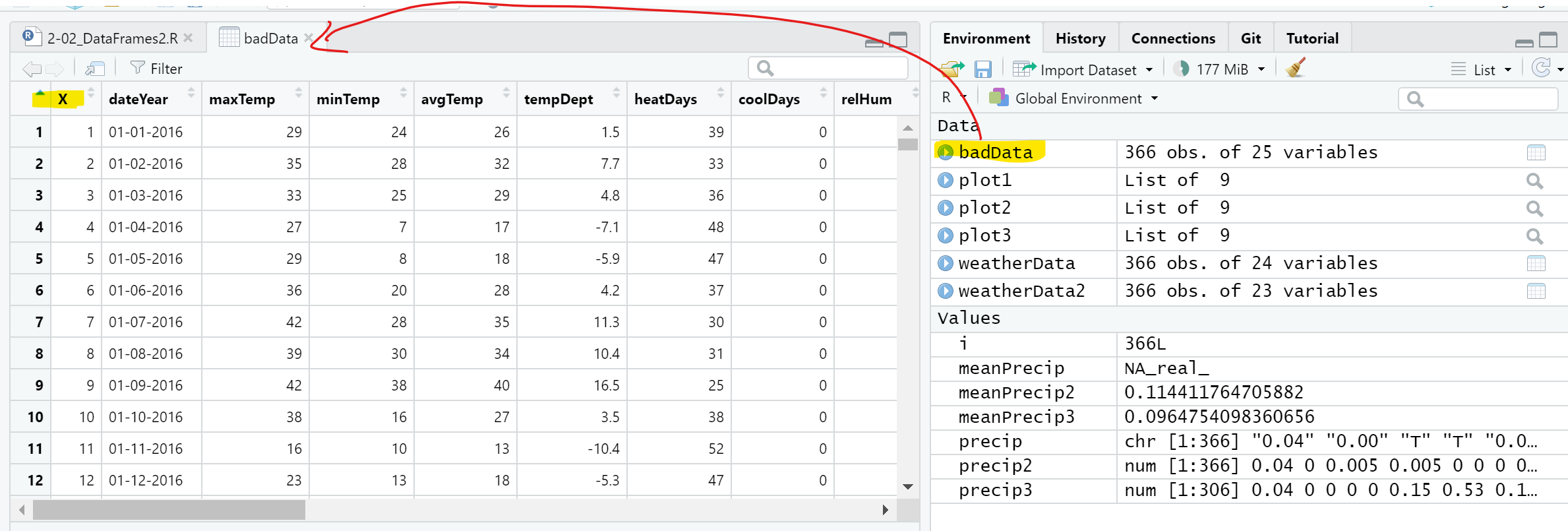
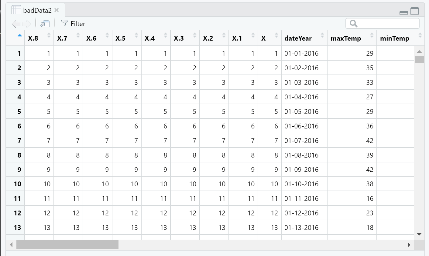
This is not a big deal but each time you write to a CSV file without setting row.names = FALSE, you create another column of row numbers to the file. If you keep writing to a CSV file without setting row.names to FALSE, you will get something like this:
4 Adding columns with the wrong number of values
While we are messing around with a throwaway data frame, let’s see what happens if you try to add/overwrite a column to the data frame that has the wrong number of values. In this case, the data frame has 366 rows, meaning there are 366 values in each column.
Let’s attempt to overwrite the column test1 with 400 values and write to a new column called test2 with 10 values:
badData$test1 = c(1:400);  # 400 values: 1-400
badData$test2 = c(1:10);   # 10 values: 1-10
The test1 line will output this error:
Error in `$<-.data.frame`(`*tmp*`, test1, value = 1:400) :
  replacement has 400 rows, data has 366
and, similarly, the test2 line will output this error:
Error in `$<-.data.frame`(`*tmp*`, test2, value = 1:10) :
  replacement has 10 rows, data has 366
Basically, R is saying that the vector you are trying to add to the data frame does not have the same number of values as the row in the data frame.
4.1 Adding column with a divisible number of values
There is one situation is which R will let you write a column to a data frame even if the number of values is not the same as the number of rows– and that is when the number of values in the vector evenly divides the number of rows in the data frame. In the case of weatherData that is any number that can evenly divide 366 (e.g., 1,2,3,6…)
In these cases, R will repeat the values provided until 366 values is reached.
So, if you use one value to create a column:
badData$test3 =10;Then R will create a column called test3 with the value 10 in every cell.
Or, if you use 6 values (366/6 = 61):
badData$test4 = c(1:6);Then R will create a column called test4 that repeat the numbers 1-6 61times:
> badData$test3
[1] 10 10 10 10 10 10 10 10 10 ...
> badData$test4
[1] 1 2 3 4 5 6 1 2 3 4 5 6 1 2 3 4 ...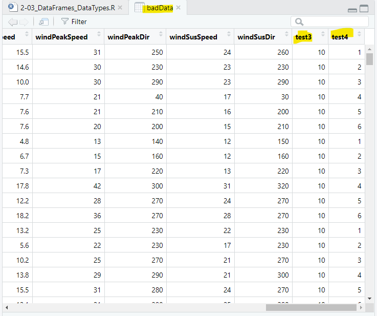
5 Manually repeating values
You can manually create a vector with repeated values using rep(), which has 2 arguments:
the value(s) you want to repeat
the number of times you want to repeat the values
If you want to repeat the letters A through F to fill a 366 value vector:
vectorAF = rep(c("A", "B", "C", "D", "E", "F"), times = 61);vectorAF repeats “A”-“F” 61 times. Let’s look at the first 20 values:
> vectorAF[1:20]
 [1] "A" "B" "C" "D" "E" "F" "A" "B" "C" "D" "E" "F" "A" "B" "C" "D" "E" "F" "A" "B"
Alternatively, you can use the argument length.out to give the length of the vector. So, if you want to repeat the numbers 1 through 10 until you reach 366 values:
vector1_10 = rep(1:10, length.out=366);If you look at the last 20 values of vector1_10, you see that the last, or 366th, value is a 6:
> vector1_10[345:366]
 [1]  5  6  7  8  9 10  1  2  3  4  5  6  7  8  9 10  1  2  3  4  5  6
If you want to repeat values a certain number and then move on to another value, for instance creating a vector with the months of the years, then you can use rep() within a vector:
firstThreeMonths = c(rep("Jan", 31), rep("Feb", 29), rep("Mar", 31));And firstThreeMonth will have 91 values:
> firstThreeMonths
 [1] "Jan" "Jan" "Jan" "Jan" "Jan" "Jan" "Jan" "Jan" "Jan" "Jan" "Jan" "Jan" "Jan"
[14] "Jan" "Jan" "Jan" "Jan" "Jan" "Jan" "Jan" "Jan" "Jan" "Jan" "Jan" "Jan" "Jan"
[27] "Jan" "Jan" "Jan" "Jan" "Jan" "Feb" "Feb" "Feb" "Feb" "Feb" "Feb" "Feb" "Feb"
[40] "Feb" "Feb" "Feb" "Feb" "Feb" "Feb" "Feb" "Feb" "Feb" "Feb" "Feb" "Feb" "Feb"
[53] "Feb" "Feb" "Feb" "Feb" "Feb" "Feb" "Feb" "Feb" "Mar" "Mar" "Mar" "Mar" "Mar"
[66] "Mar" "Mar" "Mar" "Mar" "Mar" "Mar" "Mar" "Mar" "Mar" "Mar" "Mar" "Mar" "Mar"
[79] "Mar" "Mar" "Mar" "Mar" "Mar" "Mar" "Mar" "Mar" "Mar" "Mar" "Mar" "Mar" "Mar"
6 Numeric and character columns
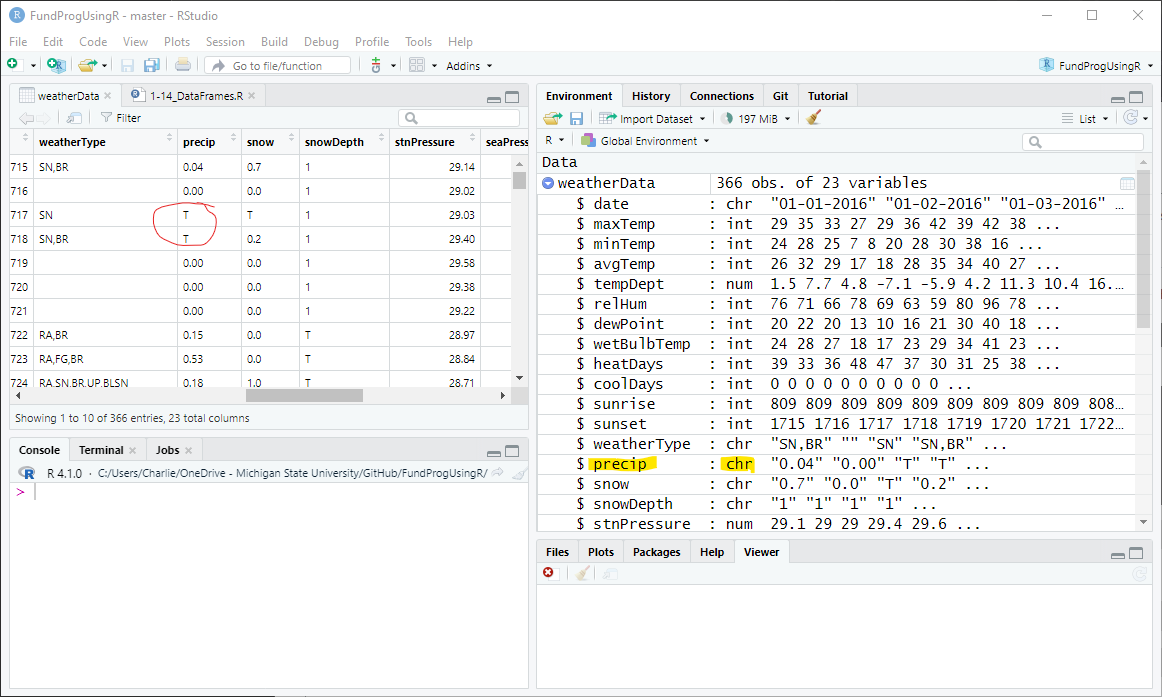
Now let’s read in the “good” CSV file created in the last lesson:
  weatherData = read.csv(file="data/Lansing2016Noaa-2.csv",
                         sep=",",
                         header=TRUE);
If we look at the Environment (Figure 4), there are a few columns in the weatherData data frame that R categorizes as string (chr) even though they are numeric by nature. For instance, precip, snow, and snowDepth are all labelled as chr even though they have (mostly) numeric values.
The issue is the “T” values used in these columns to indicate a trace of precipitation (less than 0.01 inches). “T” is a chr/string values and, in R, if any value in a vector or a column is a string then every value in the vector (or column) is treated as a string.
Note: You can also use the typeof() function to find the data type for a vector:
> typeof(weatherData$precip)
[1] "character"
6.1 When numbers are treated as characters
In R, “1234” is not the same as 1234. The former is 4 characters, a “1” followed by a “2” followed by a “3”, followed by a “4”. The latter is the number 1234. In R, you cannot perform mathematical operations on characters, even if they look like numbers.
If you try to perform mathematical operations on character, even ones that look like numbers, you will get the error: non-numeric argument to binary operator.
We can see this in the Console:
> a = 9
> b = "7"
> a + a
[1] 18
> a + b
Error in a + b : non-numeric argument to binary operator
> b + b
Error in b + b : non-numeric argument to binary operator
Let’s save the precip column in weatherData to a vector called precip
precip = weatherData$precip;A similar error will occur if you try to perform mathematical functions on precip, like adding up all of the values using sum():
> totalPrecip = sum(precip);
Error in sum(precip) : invalid 'type' (character) of argument
And statistical function like mean() will generally give an answer of NA:
> meanPrecip = mean(precip);
Warning message:
In mean.default(precip) : argument is not numeric or logical: returning NA
6.2 Forcing characters to become numbers
The solution is to change the chr (string) vector into a numeric vector using as.numeric():
Let’s use as.numeric() on the precip vector as save the results to precip2:
precip2 = as.numeric(precip);If we look at the Environment, we can see that precip2 is a numeric vector and the numbers no longer have quotes around them. But, the non-numeric “T” values were replaced with NA:
precip:   chr[1:366]  "0.04" "0.00" "T" "T" "0.00"
precip2:  num[1:366]  0.04 0 NA NA 0
6.3 Double values are numeric…
Using typeof() to find out what type of vector precip2 is:
> typeof(precip2)
[1] "double"
A double value is a numeric value. double refers to how big of a numeric value the vector can hold and meant a lot more in the days when computer memory was at a premium.
7 Operations on NA values
To R, NA means that the value is Not Available. NA can be an error indicating that an operation could not be performed and therefore no value can be given. NA could also be a placeholder for a value that is known to not exist.
NULL and NA are often confused but they are functionally much different. If NULL is used in a vector, it will remove the value from the vector:
> c(1, NULL, 3, 4, 5)
[1] 1 3 4 5
> c(1, NA, 3, 4, 5)
[1]  1 NA  3  4  5
If you try to perform mathematical or statistical operation on a vector that has numeric NA values, R will tell you the answer is NA, or NA_Real, which is just R’s way of telling you that the answer would be a real number if the NA values existed.
meanPrecip = mean(precip2);
totalPrecip = sum(precip2);meanPrecip: NA_Real
totalPrecip: NA_Real7.1 Comparing NA to NULL
NA values are, in a sense, placeholder values for data that should exist but is unknown. Therefore are mathematical and statistical operations on NA will result in NA:
> length(c(10, NA, NA, 20))
[1] 4
> sum(c(10, NA, NA, 20))
[1] NA
> mean(c(10, NA, NA, 20))
[1] NA
Whereas the NULL values will be treated as if it does not exist:
> length(c(10, NULL, NULL, 20))
[1] 2
> sum(c(10, NULL, NULL, 20))
[1] 30
> mean(c(10, NULL, NULL, 20))
[1] 15
7.2 Finding the number of NA values
is.na(precip2) will go through each value in precip2 and create a TRUE/FALSE vector with 366 values:
> is.na(precip2)
  [1] FALSE FALSE  TRUE  TRUE FALSE FALSE FALSE FALSE FALSE FALSE FALSE FALSE FALSE
 [14] TRUE FALSE  TRUE  TRUE FALSE  TRUE  TRUE FALSE  TRUE  TRUE FALSE FALSE FALSE
 ...
The TRUE values represent NA values. We can count the TRUE values using sum():
> sum(is.na(precip2))
[1] 60
So, there are 60 NA values in precip2.
7.3 Removing NA values
You can get around the NA issues by instructing R to remove the NA values from the calculation by setting the NA removal argument available in most mathematical and statistical function, na.rm, to TRUE:
meanPrecip2 = mean(precip2, na.rm = TRUE);
totalPrecip2 = sum(precip2, na.rm = TRUE);
Without the NA values in the vector, the results are:
meanPrecip2: 0.1144...
totalPrecip2: 35.01
Note: na.rm=TRUE effectively changes an NA to a NULL
7.4 Replacing the NA values
Using the argument na.rm=TRUE assumes that the NA values should be ignored. However, that is not true in this case – the NA values are the old T values and represented a trace or rain. We need to keep these values in the vector. Since a trace of precipitation is defined as less than 0.01 inches of precipitation – so we will go halfway and change all NA values to 0.005:
We will first make another copy of precip:
precip3 = precip2; # make another copy of precipAnd then cycle through all the values in precip3, checking for NA values and changing them to 0.005:
for(i in 1:length(precip3)) # go through every value in precip
{
  if(is.na(precip3[i]))     # if the value is NA
  {
    precip[i] = 0.005;      # change it to 0.005
  }
}
And we can see that precip3 now has 0.005 in place of NA:
precip3 num [1:366] 0.04 0.00 «0.005» «0.005» 0.00...7.5 Reserved Words in R
NA is a reserved word in R. This means you cannot create a variable named NA in R:
> NA = 2
Error in NA = 2 : invalid (do_set) left-hand side to assignment
NA is not the same as the string value “N” followed by “A”, so this if statement will not work:
if(precip3[i] == "NA") # checking for the characters "N" and "A"And NA is not a variable name in R, so this if statement does not work:
if(precip3[i] == NA) # checking for the variable named NAInstead, we must use the function is.na() to check for NA values:
if(is.na(precip3[i])) # checking if precip[i] is an NA valueNote: There are many other reserved words in R like NULL, TRUE, FALSE, for, if, else, function…
7.6 Mathematical operations on the new vector
Let’s find the mean and the sum of the precip3 vector with 0.005 in place of NA,
meanPrecip3 = mean(precip3);
totalPrecip3 = sum(precip3);
Adding 60 days with trace precipitation increased the sum by a little bit and lowered the mean a bit:
meanPrecip2:   0.1144...
totalPrecip2:  35.01
meanPrecip3:   0.0964...
totalPrecip3:  35.31...
7.7 Adding the numeric precip column
We will add the numeric precip3 column to weatherData and call the new column precipNum:
weatherData$precipNum = precip3;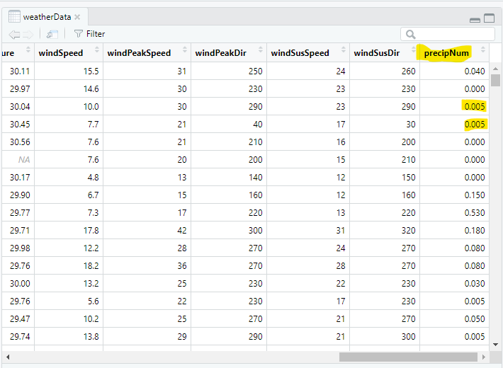
8 Plotting rainfall values
We are going to do some basic plots with the rainfall values. For all of these plots we are going to plot rainfall vs. the day number (e.g., 1 is Jan 1, 2 is Jan 2, 366 is Dec 31). We will deal with dates in a later lesson.
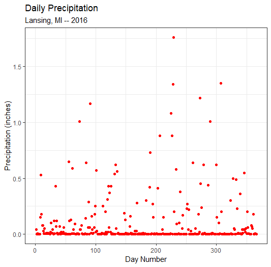
8.1 A scatterplot
The first plot will be a scatterplot with rainfall (precipNum) on the y-axis and day number on the x-axis. Since day number is just the row number, we will map the y-axis to a sequence from 1 to the number of rows in weatherData (i.e., 366)
plot1 = ggplot(data=weatherData ) +
  geom_point( mapping=aes(x=1:nrow(weatherData),  # 1:366
                          y=precipNum),
              color = "red") +
  labs( title="Daily Precipitation",
        subtitle="Lansing, MI -- 2016",
        x = "Day Number",
        y = "Precipitation (inches)") +
  theme_bw();
plot(plot1);
Note: we could have used 366 instead of nrow(weatherData) but nrow(weatherData) is more robust as it can handle changes to the size of the data frame (e.g., a year that is not a leap year)
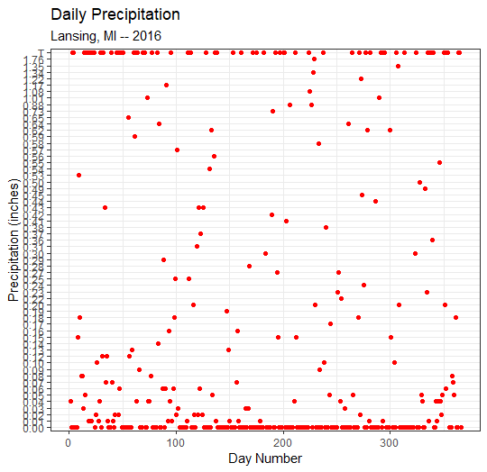
8.2 Scatterplot with chr values
GGPlot can also create a scatterplot from the precipitation values that are given in the precip column that is of type chr:
  plot2 = ggplot(data=weatherData ) +
    geom_point( mapping=aes(x=1:nrow(weatherData),
                            y=precip),  # chr values
                color = "red") +
    labs( title="Daily Precipitation",
          subtitle="Lansing, MI -- 2016",
          x = "Day Number",
          y = "Precipitation (inches)") +
    theme_bw();
  plot(plot2);
But, since precip contains chr/string values (i.e., not numbers), GGPlot will output every unique precip value on the y-axis and put them in “alphabetical” order. This is why T is at the top of the y-axis – T is alphabetically greater than the numbers.
9 Application
1) Answer the following questions in comments at the top of your script:
In the weatherType column, there are a bunch of days without any conditions. Would either NULL or NA be appropriate to use in those cells? Explain.
What happens when you try to sum, using sum(), the following two vectors? Why?
c(8, 10, 6, NULL, 4)
c(8, 10, 6, NA, 4)
2) Find the total amount of snow was for the year and save it to the variable named snowTotal
- the snow column also uses T values, but trace in this case means snowfall between 0 and 0.5 inches
3) Find the average snow depth for the year and save it to the variable snowDepthAvg
4) Create a vector with 366 values called seasons and add the vector to a column in the weatherData called season
March 21 June 21, and September 21 are approximate dates for the transition of the season – it is OK for this application to be off by a few days
But, you need to deal with the fact that the beginning of the year and end of the year are winter days
5) Create a vector call daysOfTheWeek (Sun-Mon-Tues-Wed) and add it to the weatherData column
- Note: January 1, 2016 was a Friday
6) Create a scatterplot with relative humidity on the y-axis and (numeric) precipitation on the x-axis.
- Color the points blue and add appropriate labels and titles
Save the script as app2-03.r in your scripts folder and email your Project Folder to Charlie Belinsky at belinsky@msu.edu.
Instructions for zipping the Project Folder are here.
If you have any questions regarding this application, feel free to email them to Charlie Belinsky at belinsky@msu.edu.
9.1 Questions to answer
Answer the following in comments inside your application script:
What was your level of comfort with the lesson/application?
What areas of the lesson/application confused or still confuses you?
What are some things you would like to know more about that is related to, but not covered in, this lesson?