1-03: Mathematical Operations

0.1 Changes

1 Purpose

• Perform mathematical operations, including powers, on numerical variables

• Explicit use of mathematical symbols in formulas

• Convert algebraic formulas to programming formulas

• Use parentheses to establish the order of operations for formulas

2 Questions about the material…

If you have any questions about the material in this lesson, feel free to email them to the instructor, Charlie Belinsky, at belinsky@msu.edu.

3 Putting a formula in code

Once again, we will calculate velocity using distance and time, except, we will now use the full version of the velocity formula, which looks at the changes in distance and time as opposed to absolute distance and time.

 

The full velocity formula is (subscript i means initial, subscript f means final):

\(v=\frac{d_{f}-d_{i}}{t_{f}-t_{i}}\) .

 

Note: If t_i and d_i are zero then you get the formula we used in Lesson 1-2: (\(\boldsymbol{v}=\frac{d}{t}\))

 

We are going to code this formula, but there are a couple of issues:

1. fractions are “stacked” – but in scripts, equations can only be read left to right

2. variable names have subscript characters (e.g., t_i), but subscript and superscript characters are not allowed in script

3.1 Minding your parentheses

In script, everything goes left-to-right so you cannot write a fraction as you would in Algebra.  Instead, we need to be more explicit and put both both the numerator and the denominator in parentheses:

\[ v=\frac{\left(d_{f}-d_{i}\right)}{\left(t_{f}-t_{i}\right)} \]

Then, pull out the fraction between the numerator and denominator and replace it with a division sign:

\[ v=\left(d_{f}-d_{i}\right) /\left(t_{f}-t_{i}\right) \]

Now the formula is all on one line, but the symbols need to be replaced with valid variable names that do not have subscripts:

\[ \text { velocity }=(\text { finalDist }- \text { initDist }) /(\text { finalTime }- \text { initTime }) \]

This is now a valid line of code in R, assuming all four variables on the right side have assigned values.

velocity = (finalDist - initDist) / (finalTime - initTime);

The line of code above says that velocity will be assigned the value equal to the calculations of the four variables on the right side of the equation.

3.2 Other ways to assign values

In most programming languages the equal sign ( = ) is used to assign values. The equal sign always evaluates what is on the right side and assigns it to the variable on the left. 

 

In R, you can also use arrows to assign values and the arrow can be on either side:

«velocity <-» (finalDist - initDist) / (finalTime - initTime); # commonly used
(finalDist - initDist) / (finalTime - initTime) «-> velocity»; # rarely used

The top ( <- ) is the most common method used to assign values in R.

The bottom method ( -> ) works but is rarely used anymore. 

I prefer using ( = ) to ( <- ) because ( = ) is used in most programming languages whereas ( <- ) is not. 

 

Note: In this case, ( = ) and ( <- ) are functionally the same. There are differences between the two, which we will talk about in the lesson on functions.

3.3 Variable naming error

Here is the full script with a small error on the line calculating velocity:

rm(list=ls());   # Clear out environment
options(show.error.locations = TRUE); # give line number of error

finalDistance = 100;
initDistance = 50;
finaltime = 20;       # misspelled: use t instead of T
initTime = 15;
# error will be on the line below:
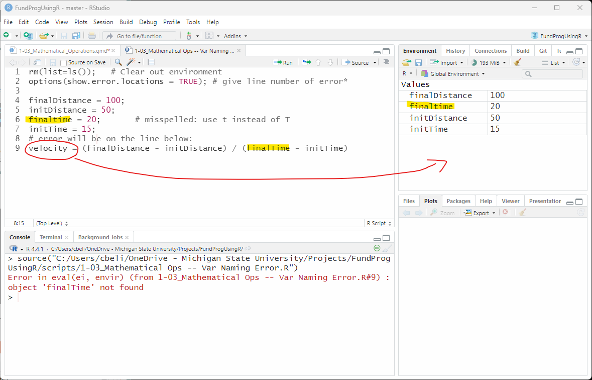
«velocity = (finalDistance - initDistance) / (finalTime - initTime)»

Every variable on the right side of the velocity equation must be given a value beforehand –  otherwise, you will get the pesky Object not found error as shown in the image below (Figure 1)

 

Figure 1: Object not found because the variable name does not exist (it is misspelled).

 

Extension: The show.error.location line

 

Note: Object is almost synonymous with Variable in R.  The error is basically saying that there is no variable with that name.  Any spelling error will cause the Object not found error.  In this case I “spelled” the variable name wrong by changing the case of the T.  finaltime is not the same as finalTime.
 

rm(list=ls());           # clean out the environment
options(show.error.locations = TRUE); # give line number of error
 
finalDistance = 100;
initDistance = 50;
«finalTime» = 20;
initTime = 15;
velocity = (finalDistance - initDistance) / (finalTime - initTime);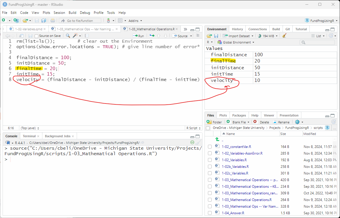

Figure 2: Misspelled variable name corrected – script now calculates velocity.

4 Powers and multiplication

We will look at one more formula that relates kinetic energy to mass and velocity:

\[ E_{k}=\frac{1}{2} m v^{2} \]

There are two new issues with coding this formula:

1. the square function is a superscript – you cannot use superscript characters in R

2. the implicit multiplication – we know that mass (m) and velocity (v) are being multiplied, but there is no multiplication sign

4.1 Dealing with parenthesis and multiplication

So let’s first pull the one-half out of fraction form and into division form:

\[ E_{k}=1 / 2 m v^{2} \]

We need to be more explicit because this formula could be misinterpreted by R as \(E_{k}=1 /\left(2 m v^{2}\right)\), so we need to put the one-half in parenthesis:

\[ E_{k}=(1 / 2) m v^{2} \]

Next, we will explicitly put in the multiplication symbols – a necessity in programming:

\[ E_{k}=(1 / 2)^{*} m^{*} v^{2} \]

Traps: Forgetting Multiplication Symbol

 

And then change the symbols to script-friendly variable names:

\[ \text { kineticEnergy }=(1 / 2)^{*} \text { mass }^{*} \text { velocity }^{2} \]

4.2 Dealing with square power

In R the ( ^ ) is the power operator.  So ^2 means raise to the power of 2 (i.e., square):

# this formula works...
kineticEnergy = (1/2)*mass*velocity^2;

While the above works correctly, it is often helpful to be explicit and add parenthesis around the value or values that are getting raised to the power:

# more explicit solution
kineticEnergy = (1/2)*mass*(velocity)^2;

5 The power operator ( ^ )

The ( ^ ) operator works for all powers including square roots, cubed roots, and mixed powers (e.g., raising to the 3/2 or 5/3).

 

Let’s rearrange the kinetic energy formula to solve for velocity, which requires a square root

\[ v=\sqrt{\frac{2 E_{k}}{m}} \]

To put the above formula into a script form, we need to:

1) Put the numerator and denominator on one line by taking out the fraction and replacing it with a division sign.

\[ v=\sqrt{\left(2 E_{k} / m\right)} \]

2) Be explicit and put in multiplication symbols.

\[ v=\sqrt{\left(2^{*} E_{k} / m\right)} \]

3) Spell the formula out using script-friendly variable names:

\[ \text { velocity }=\sqrt{\left(2^{*} \text { kineticEnergy / mass }\right)} \]

4) Use the power operator ( ^ ) to square root the whole formula.  Square rooting something is the same as saying raise it to the 1/2 power. Since we are square rooting the whole formula, we need to put the whole formula in parenthesis.

\[ \text { velocity }=\left(2^{*} \text { kineticEnergy } / \text { mass }\right)^{1 / 2} \]

5.1 Coding the power

So we have this in R:

rm(list=ls());          # clean out the environment

kineticEnergy = 50;
mass = 5;
velocity = (2*kineticEnergy / mass)^1/2; # still a problem here!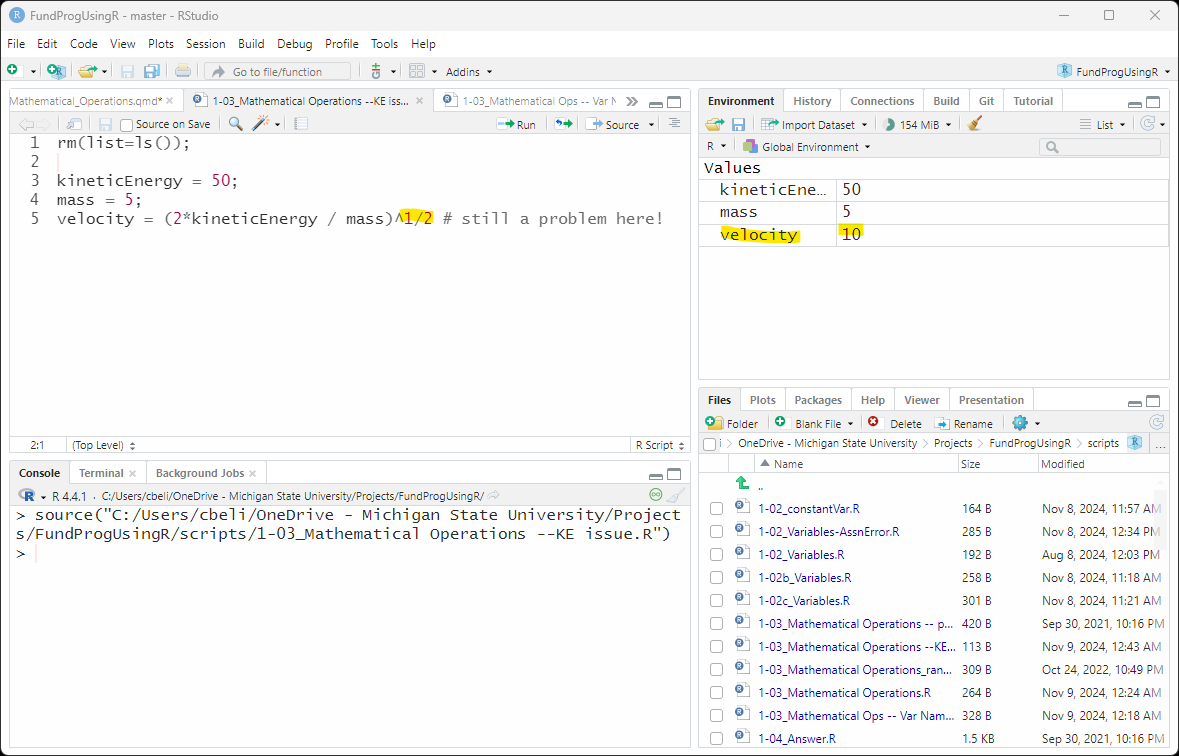

Figure 3: Incorrect answer for velocity because the power is missing parentheses

5.2 Correcting the power with parentheses

The Environment tab (Figure 3) shows that v is, unexpectedly, 10.  This is because of the order-of-operations. Instead of raising the (2*kineticEnergy/mass) to the 1/2 power, the above code raised (2*kineticEnergy/mass) to the first (1) power and then divided everything by 2.  We need to be more explicit and put the 1/2 in parenthesis.

rm(list=ls());          # clean out the environment

kineticEnergy = 50;
mass = 5;
velocity = (2*kineticEnergy / mass)^«(1/2)»; # now we are good!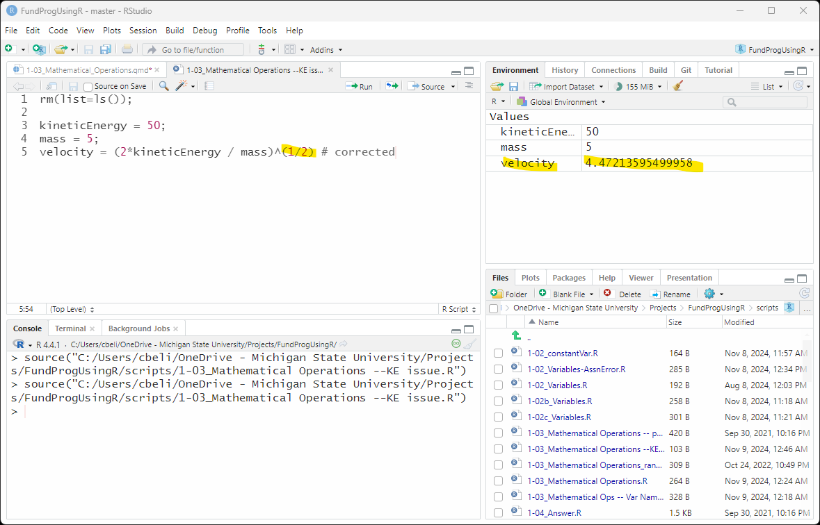

Figure 4: Correct answer for velocity

5.3 More power and roots

This method will work for all powers and roots:

rm(list=ls());          # clean out the environment

kineticEnergy = 50;
mass = 5;

test1 = (2*kineticEnergy / mass)«^(1/3)»;  # third root
test2 = (2*kineticEnergy / mass)«^(5)»;    # fifth power
test3 = (2*kineticEnergy / mass)«^(5/3)»;  # mixed root and power
test4 = (2*kineticEnergy / mass)«^(3.17)»; # decimal power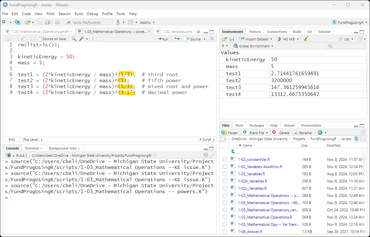

Figure 5: Testing different powers in R

6 The square root function

In R, you will usually see square roots done using the sqrt() function:

velocity = «sqrt»(2*kineticEnergy / mass);  # how square roots are usually done

sqrt() works just fine but there is no equivalent for all the other powers and roots.  That is why I prefer to use the ( ^ ) operator – it is easy to remember and you can use it everytime you need a power or a root.

velocity = (2*kineticEnergy / mass)^(1/2); # how I prefer to do them

7 Mathematics on multiple lines

You need to be careful when putting mathematics on multiple lines in R. For instance if you command:

num = 1 + 1 + 1 + 1
      + 1 + 1 + 1;

will set num = 4 because R thinks that num = 1 + 1 + 1 + 1 is the complete command.

 

If the command is meant to go to the next line, you need to give R a reason to continue to the next line. This can be done by moving the operation to the end of the line so that R looks on the next line for the operand:

 num = 1 + 1 + 1 + 1 + 
       1 + 1 + 1;

Or by wrapping the values in parentheses so that R knows it needs to continue until the end parenthesis is found:

num = (1 + 1 + 1 + 1 
       + 1 + 1 + 1);

The latter two examples will both set num = 7.

8 Random values

In Figure 5 we hardcoded the values for kineticEnergy and mass. Harcoded means we directly provided a values for the two variables.  Now we will randomly pick values for variables using sample().

 

sample() requires two arguments:

• the range of numbers you want to randomly sample from

• the number of values you want to randomly sample (for now we will just do one value)

 

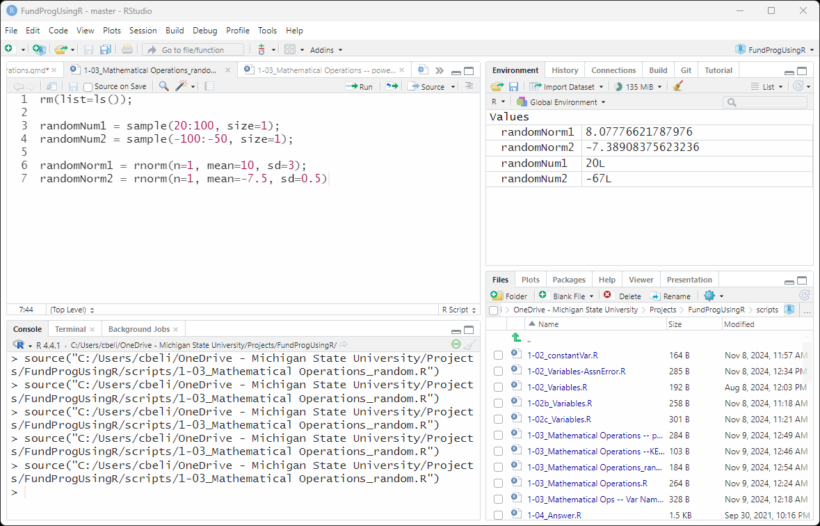
The code to pick one random number between 20 and 100 is:

randomNum1 = sample(20:100, size=1);

note: 20:100 is inclusive of the numbers on both ends – so, 20 and 100 are both possibilities meaning there are 81 possible numbers to choose randomly from

 

The code to pick a random number between -100 and -50 is:

randomNum2 = sample(-100:-50, size=1);

sample() always returns an integer – in the above case there are 151 possible integers between -100 and 50.  

8.1 normal values

sample() gives every number an equal chance.  If there are 100 numbers in the range then every number has a 1% chance of being picked.  If you want to pick a random value, but weigh the value (e.g., a normally distributed random values) then you can use rnorm().

 

rnorm() requires three arguments:

• the number of values you want to randomly pick (for now, we will just choose 1 value)

• the mean of the normal distribution you want to pick randomly from

• the standard deviation of the normal distribution

 

The code to pick one random number from a normal distribution with mean 10 and standard deviation 3 is:

randomNorm1 = rnorm(n=1, mean=10, sd=3);

The code to pick one random number from a normal distribution with mean -7.5 and standard deviation 0.5 is:

randomNorm2 = rnorm(n=1, mean=-7.5, sd=0.5);

rnorm() always returns a decimal number

Figure 6: Picking random numbers – the random numbers will be different each time you execute the code

9 Application

1) Add this code right after the rm(list=ls()) lines:

set.seed(5); 

The above line will make sure that you get the same “random” number every time you execute your script by creating a seed value.  Seed values are covered in a much later lesson.

 

2) Create six variables that all hold length values:

• 1st and 2nd are assigned the values: 25, 30

• 3rd and 4th are randomly picked between 20 and 30 (each number has an equal chance)

• 5th and 6th are randomly picked from a normal distribution with mean of 25 and standard deviation of 2

 

3) Calculate the (a) mean, (b) variance, and (c) standard deviation of the six values.

• Visit this page if you need a reminder about how to calculate mean, variance, and standard deviation

• you can use R functions like mean(), var(), and sd() to check these values, but I want you to manually solve these – it is important to learn how to properly code the mathematics because you will often not have functions to do it for you.

• Extension: Mathematical operations across multiple lines

 

4) Make sure the 6 values, their mean, their variance, and their standard deviation appear in the Environment tab after the script is executed.

 

5) Challenge: Pick a random two-digit decimal number between 0 and 1 (e.g., 0.23, 0.89, 0.10)

• each two-digit decimal number should have an equal chance of being chosen
• neither sample() nor rnorm() can solve the problem by itself – you need to use one of them and then mathematically manipulate the result

 

 

Save the script as app1-03.r in your scripts folder and  email your Project Folder to Charlie Belinsky at belinsky@msu.edu.

 

Instructions for zipping the Project Folder are here.

 

If you have any questions regarding this application, feel free to email them to Charlie Belinsky at belinsky@msu.edu.

9.1 Questions to answer

Answer the following in comments inside your application script:

1. What was your level of comfort with the lesson/application?

2. What areas of the lesson/application confused or still confuses you?

3. What are some things you would like to know more about that is related to, but not covered in, this lesson?

10 Extension: Mathematical operations across multiple lines

If you have a long mathematical formula to execute in code, there is a good chance that you will want to break the code up into multiple lines.

 

To keep it simple, let’s add 5 values together across multiple lines:

c1 = 10 + 10 + 10 +
     10 + 10;

If you put the above code in you script, then you will get c1 = 50 in the Environment.

 

However, this code:

c2 = 10 + 10 + 10
     + 10 + 10;

will put c2=30 in the Environment.

 

This is because R did not know the continue the equation for c2 to the second line.  R treated the first line as the complete command/equation.  By putting the ( + ) at the end of the first line for c1, R knew it needed to continue the command on the next line.

 

By the way, R does do something with the second line for c2 – it prints the answer to Console if you click Run:

> c2 = 10 + 10 + 10
>      + 10 + 10;
[1] 20

In other words:

+ 10 + 10

is a command that evaluates to 20

11 Traps: Forgetting Multiplication Symbol

Let’s say you are solving for kinetic energy:

\[ E_{k}=\frac{1}{2} m v^{2} \]

And you have a value for velocity (v) and mass (m)

rm(list=ls());          # clean out the environment

m = 100;
v = 10;
«KE = ????;    # should be: KE = (1/2)*m*v^2;»

If you code KE like this::

KE = 1/2*mv^2;

Then you will get the error: object ‘mv’ not found in the Console tab because R does not realize you want to multiply the variables m and v, R thinks you are trying to use a variable named mv, and the variable mv does not exist.

 

If you code KE like this::

KE = (1/2)m*v^2;  # same error arises if you do 1/2m*v^2

you will get the error: unexpected symbol (Figure 7) and the Console tab will point to the m

Figure 7: Unexpected symbol error

 

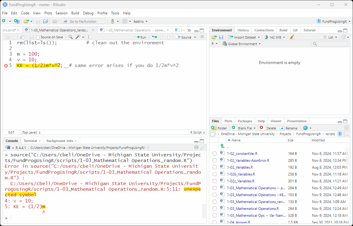
In this case, R is expecting an operation after (1/2) – R does not assume multiplication.  m is a variable, not a operation, hence the unexpected symbol error.

12 Trap: Units, or lack thereof, in programming

One problem that crops up quite often in programming is that none of the numbers used in calculations have units.  So we often have lines of code without any mention of units like this:

# find an average of the following three weights
weight1 = 175;
weight2 = 200;
weight3 = 210;

aveWeight = (weight1 + weight2 + weight3) / 3;

And if we add units to the number…

# find an average of the following three weights
«weight1 = 175lb;  # causes "unexpected symbol" error»
weight2 = 200lb;
weight3 = 210lb;

aveWeight = (weight1 + weight2 + weight3) / 3;

We get the error unexpected symbol because R is expecting some sort of operation after the number 175 and lb is not a valid operation. 

 

Note: Lines 3 and 4 would also cause an unexpected symbol error but R ceases executing at the first error.

 

It is best to mention the units somewhere in the comments especially if your script is large or others are using your script.

# find an average of the following three weights («all in pounds»)
weight1 = 175;
weight2 = 200;
weight3 = 210;

aveWeight = (weight1 + weight2 + weight3) / 3;

Otherwise, you risk a situation like the Mars Climate Orbiter crash, which could have easily been avoided with proper comments.

13 Extension: The show.error.location line

The second line of code in Figure 1 tells R to provide the line number where an error occurs:

options(show.error.locations = TRUE);

In Figure 1, the Console tab message indicates the error is at line 9 because of the options() command above. This seems like a great idea except that this command only works in very limited situations, not enough for me to justify keeping it in the script.

 

Unfortunately, R is one of the harder programming languages to debug. We will get to some debugging strategies in later lessons. For now, you can include the show.error.location line in your code. It does not hurt – it just has limited utility.